Surface temperatures across Earth’s poles pulse with the seasons, as seen in this animation based on two years of data collected by NASA’s PREFIRE (Polar Radiant Energy in the Far-InfraRed Experiment) mission.
NASA/Chad Greene
At the top and bottom of the planet, the seasons arrive on a schedule all their own. Satellite data from a mission measuring infrared energy reveal just how differently—and how dramatically—surface temperatures swing across two full years at the poles.
In this animation, surface temperatures across the Arctic and Antarctic pulse between cold (dark blue) and milder to warm (lighter blue to red). Data for the animation come from NASA’s PREFIRE (Polar Radiant Energy in the Far-InfraRed Experiment) satellites. The mission’s twin CubeSats began collecting science data in July 2024 and have now captured two complete seasonal cycles at each pole.
Because the two poles sit in opposite hemispheres, their seasons occur at opposite times—and the swing between seasons differs, too. In the Arctic, cold, dark winters give way to summers warm enough to thaw vast stretches of tundra and sea ice. In Antarctica, Earth’s coldest continent, summer temperatures rarely climb above freezing before the bitter cold of winter returns.
Surface temperatures, and how they fluctuate, offer a window into Earth’s energy budget, the net flow of energy into and out of the Earth system. Sunlight absorbed by the surface is re-radiated as infrared heat, which bounces between Earth’s surface and atmosphere before escaping to space. The poles play an important role in this process. Atmospheric and ocean circulation carries excess heat absorbed in the tropics toward the poles, where it radiates away to space, helping regulate the planet’s temperature.
“By measuring invisible heat radiating from Earth’s coldest places, PREFIRE is helping scientists understand why the poles are changing so rapidly, and what those changes might mean for the rest of the planet,” said Chad Greene, a glaciologist at NASA’s Jet Propulsion Laboratory.
Scientists have long known that far-infrared radiation accounts for nearly 60 percent of the energy Earth loses to space, but that portion of the spectrum—invisible to human eyes—had never been comprehensively measured on a global scale. By directly tracking this invisible energy in near-real-time, the PREFIRE mission is helping scientists refine models and gain a better understanding of the Earth system.
“Weather systems, river flows, shipping routes, and ice sheet stability are all influenced by energy movement in a part of the spectrum that only PREFIRE can see,” said Tristan L’Ecuyer, an atmospheric scientist at the University of Wisconsin-Madison and principal investigator of the PREFIRE mission. “Now that the invisible has been made visible, we can begin to improve weather and climate predictions that industries, our national defense, and Arctic communities rely on.”
Maps courtesy of Chad Greene, NASA/JPL, using data from NASA’s PREFIRE mission. Story by Kathryn Hansen.
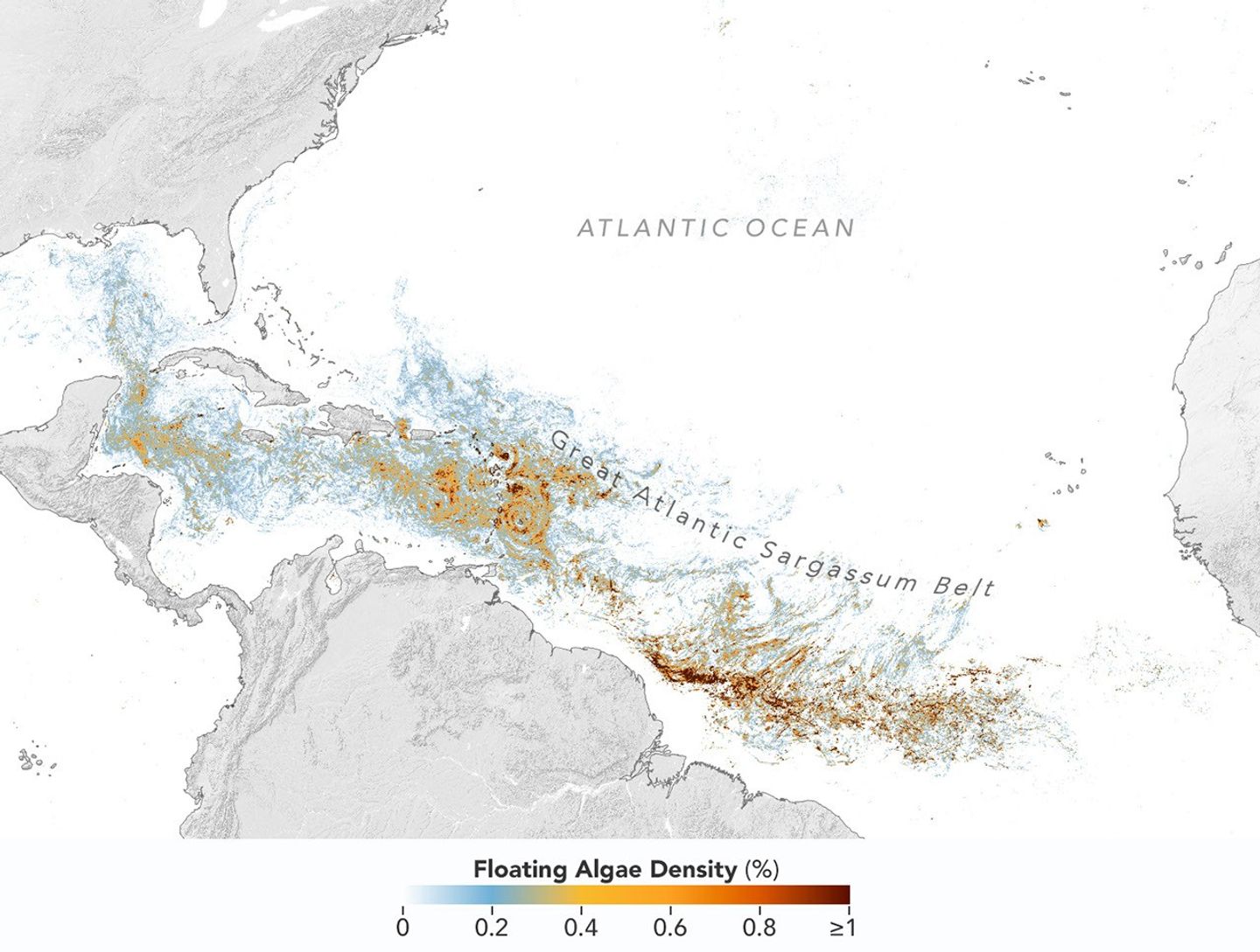
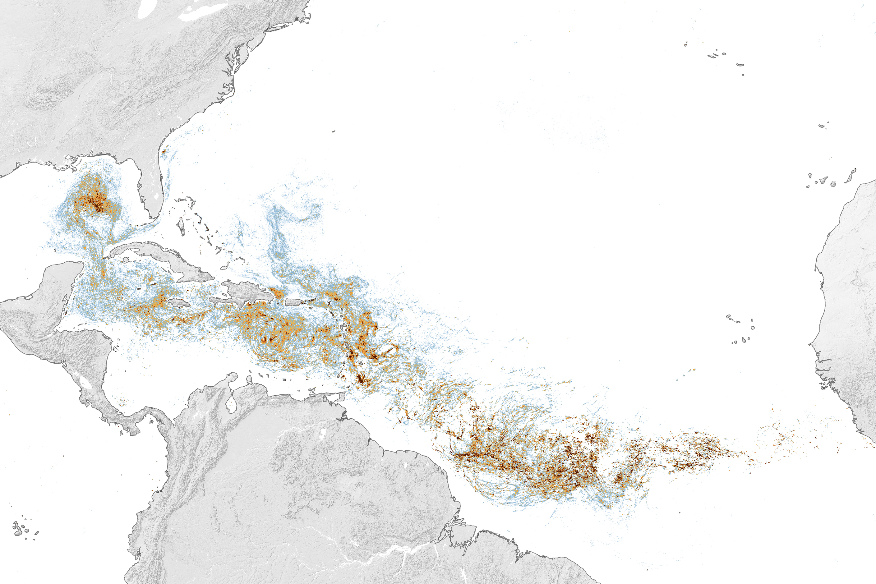
This map, based on data from the OCI (Ocean Color Instrument) on NASA’s PACE (Plankton, Aerosol, Cloud, ocean Ecosystem) satellite, shows Sargassum highly concentrated in the tropical Atlantic in June 2026.
NASA Earth Observatory/Lauren Dauphin
Sargassum, a type of brown floating algae, has shifted its range in recent decades, thinning out in the North Atlantic’s Sargasso Sea while proliferating in the tropical Atlantic. That trend, underway since 2011, continued in 2026 as the algae, commonly known as a type of seaweed, reached its annual peak in June across a stretch of ocean known as the Great Atlantic Sargassum Belt.
The belt’s Sargassum abundance in June 2026 made it the second-highest Sargassum year in the satellite record, slightly behind 2025, according to scientists at the University of South Florida (USF) College of Marine Science. Regionally, the Caribbean Sea and the Gulf of America (Gulf of Mexico) both hit record highs, according to USF’s June 2026Sargassum outlook. The western and eastern Caribbean saw 3.6 and 9 million metric tons, respectively, while the Gulf saw 5 million metric tons—nearly double its previous record, also set in 2025.
“The belt is a basin-scale phenomenon that can have devastating local-scale impacts throughout the Caribbean and Gulf, and satellite observations are the only method that captures both scales on a daily basis,” said Brian Barnes, a marine scientist at the Optical Oceanography Laboratory at USF. “The tracking done by our lab helps communities know the current extent of Sargassum and prepare for what’s to come.”
In moderate amounts in the open ocean, Sargassum provides habitat for turtles, invertebrates, fish, and birds, and adds oxygen to the water through photosynthesis. But too much of it near shore can tangle and suffocate marine life, and mats that sink can smother corals and seagrasses. On beaches, decomposing Sargassum releases hydrogen sulfide, a rotten-egg-smelling gas that’s a potential problem for both ecosystems and tourism.
The map above shows Sargassum density in the tropical Atlantic Ocean in June 2026. Red and orange areas are where Sargassum densities were the highest. Note that although the “belt” appears continuous, discrete Sargassum mats are scattered across the ocean surface. The map is based on satellite measurements of how much of the ocean surface was covered by the seaweed, averaged per pixel across all observations made in June by the OCI (Ocean Color Instrument) on NASA’s PACE (Plankton, Aerosol, Cloud, ocean Ecosystem) satellite.
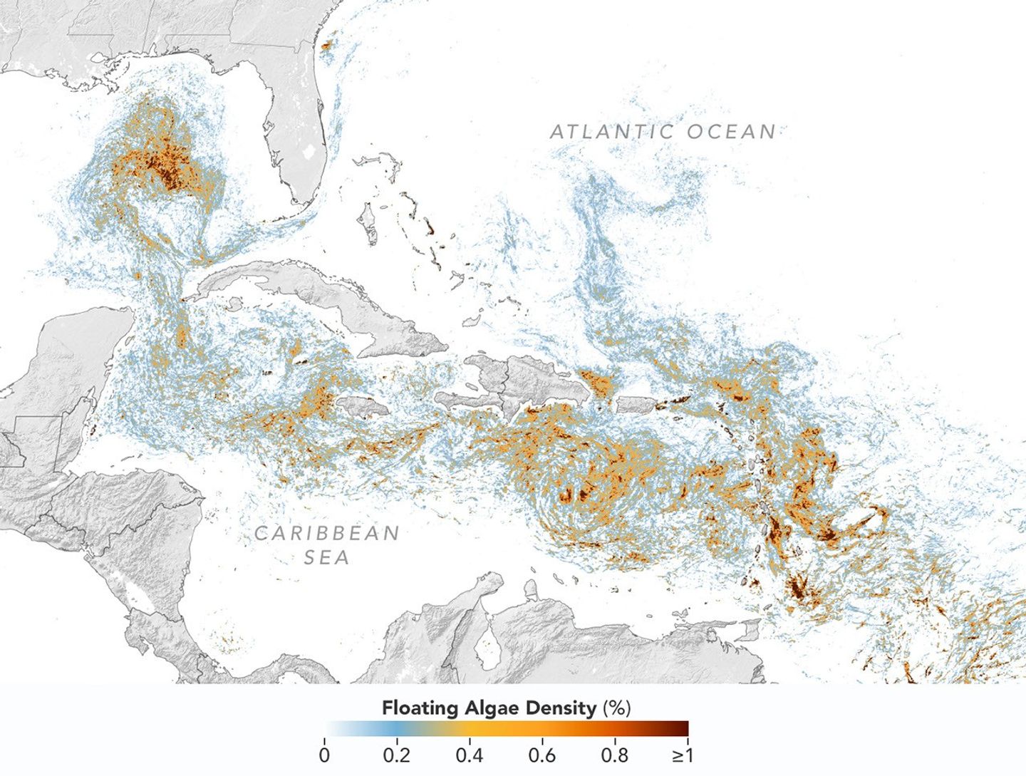
This detailed view of the same PACEOCI map highlights Sargassum concentrations across the Caribbean Sea and Gulf of America, both of which saw record-high amounts of the floating algae in June 2026.
NASA Earth Observatory/Lauren Dauphin
Ocean currents and winds shape the Sargassum belt, which, despite the patchiness, stretches nearly continuously from West Africa to the Gulf and holds a fairly steady “width” from the western tropical Atlantic westward, explained Chuanmin Hu, also an optical oceanographer at USF. The ocean currents have also spared Florida’s west coast from inundation this summer, while delivering large amounts of seaweed to the Florida Keys and the state’s east coast. The bulk of the Sargassum, however, is visible in the Caribbean Sea, shown in detail above, where problems associated with inundation have been more severe, Hu said.
Data for the maps were provided by Lin Qi, an oceanographer at NOAA’s Center for Satellite Applications and Research, who has been working to generate Sargassum maps based on data from PACE, which was launched in February 2024. The work extends that of Qi and colleagues at USF’s Optical Oceanography Laboratory. This team first developed Sargassum detection techniques using MODIS (Moderate Resolution Imaging Spectroradiometer) on NASA’s long-running Terra and Aqua satellites and VIIRS (Visible Infrared Imaging Radiometer Suite) on the NOAA-20 satellite—data that have been a key component of USF’s Sargassum Watch System and of research into the seaweed’s longer-term trends.
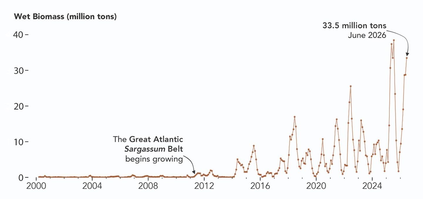
Satellites detect Sargassum by its signals in reflected sunlight. Because of its plant structure and chlorophyll pigments, Sargassum reflects more near-infrared light than water. Scientists flag pixels where the reflectance spikes above the levels produced by plain seawater, and then they use the strength of this spike to estimate Sargassum density, which refers to the fraction of ocean surface covered by the seaweed in each pixel. Density estimates can then be converted into biomass, or the total weight of Sargassum present within a pixel, which is how the longer-term trends in the chart below are tracked.
NASA Earth Observatory/Lauren Dauphin
The chart above uses the continuous MODIS record since March 2000 to show how Sargassum biomass across the Great Atlantic Sargassum Belt has changed through June 2026. Notice the uptick beginning around 2011, when the belt was first developing, and the seasonal dips in winter and peaks in spring and summer. The record high in July 2025 stands out, followed by the quick rise in early 2026—especially in the first four months of the year—that culminated in the year’s peak in June. More recent observations, not yet reflected in the chart, indicate Sargassum biomass declined through the following month of July.
“Since the initial appearance of the Great Atlantic Sargassum Belt in 2011, the total Sargassum amount in the Atlantic Ocean has increased substantially, more than doubling every five years,” Hu said. He added that the exact mechanism is still being investigated, but it’s possibly related to ocean warming, multiple nutrient sources, and the fact that large Sargassum mats attract other organisms—such as nitrogen-fixing bacteria—that can supply additional nutrients to sustain further growth.
Alongside data from MODIS and VIIRS, OCI data from PACE now feeds into the Sargassum Watch System’s near-real-time daily and weekly composite maps. A recent study of the central-west Atlantic led by Qi, spanning May through August 2024, found that OCI offers several advantages over its predecessors, observing more of the ocean and detecting Sargassum with greater sensitivity.
Hu noted that the added pixels from OCI can improve near-real-time monitoring and analyses of short-term fluctuations. And its higher sensitivity, he said, will also lead to improved maps during winter months, “thus helping understand Sargassum changes over time.”
Additionally, the study’s authors found that OCI’s hyperspectral capability makes it the only sensor able to spectrally discriminate Sargassum pixels across the Atlantic Ocean “without ambiguity,” adding confidence to the interpretation of detected image features—especially in parts of the Atlantic where another type of floating algae, Trichodesmium, has been reported.
“I think I can speak for all project members, past and present, in sharing how rewarding it is to see the promise of PACE’s advancements come to life,” said Jeremy Werdell, PACE project scientist at NASA’s Goddard Space Flight Center. “OCI has started a true renaissance in aquatic ecosystem monitoring from space.”
NASA Earth Observatory maps and chart by Lauren Dauphin, using PACE and MODIS data courtesy of Lin Qi (NOAA), and Brian Barnes and Chuanmin Hu (University of South Florida, Optical Oceanography Laboratory). Story by Kathryn Hansen.
Smoke pours from dozens of large fires in Oregon in this image captured by MODIS (Moderate Resolution Imaging Spectroradiometer) on NASA’s Aqua satellite on July 26, 2026.
NASA Earth Observatory/Michala Garrison
Dry thunderstorms that popped up over the Cascade Range on the evening of July 15, 2026, peppered Oregon and Washington with thousands of lightning strikes as they moved east across the states. By the following day, NASA satellites had begun to detect large numbers of wildland fires burning throughout central and eastern Oregon.
Though initially small, these blazes strengthened as they were fanned by gusty winds and raced through landscapes parched by extreme drought and baking in summer heat. When NASA’s Aqua satellite captured the image shown above on the afternoon of July 26, smoke poured northeast from dozens of large fires that had collectively charred hundreds of square miles. The fires produced a blanket of haze, prompting state officials to issue air quality advisories for eastern Oregon.
Many communities faced evacuation orders as more than 10,000 firefighters battled wildfires throughout the state. On the day the image was captured, the largest active fires were the Hay Creek Complex, Brewer, Big Grass, Akawa Butte, and Powder River fires. Several of these blazes were less than 5 percent contained, according to the National Interagency Fire Center. State officials invoked Oregon’s Emergency Conflagration Act to protect communities as they responded to particularly threatening fires such as the Shingle, Bench, Beachcomb, and Second Flat fires.
Government satellite data are part of a global system of observations used to track fire behavior and analyze emerging trends. Among the real-time wildfire monitoring tools that NASA makes available are FIRMS (Fire Information for Resource Management System), the Worldview browser, and the Fire Event Explorer.
As of July 27, 2026, fires in Oregon had burned more than one million acres, according to news outlets. Meanwhile, the National Interagency Fire Center reported that fires had burned more than 4 million acres across the United States. The 10-year average (2016-2025) for this point in the season is 3.4 million acres.
NASA Earth Observatory image by Michala Garrison, using MODIS data from NASA EOSDIS LANCE and GIBS/Worldview.Story by Adam Voiland.
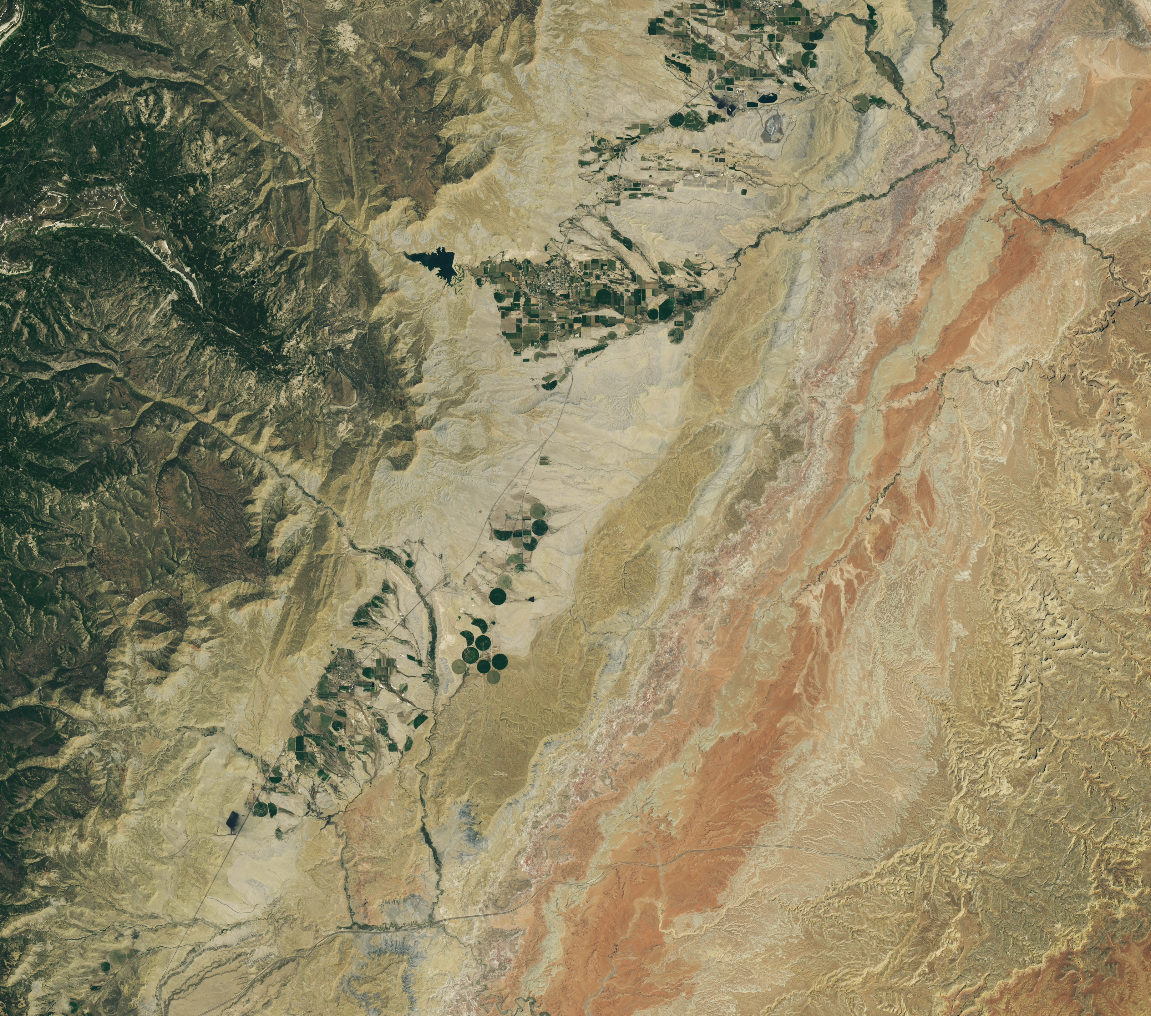
A dry, tan-colored valley containing a few circular irrigated fields runs roughly north-south through the image.
NASA Earth Observatory / Lauren Dauphin
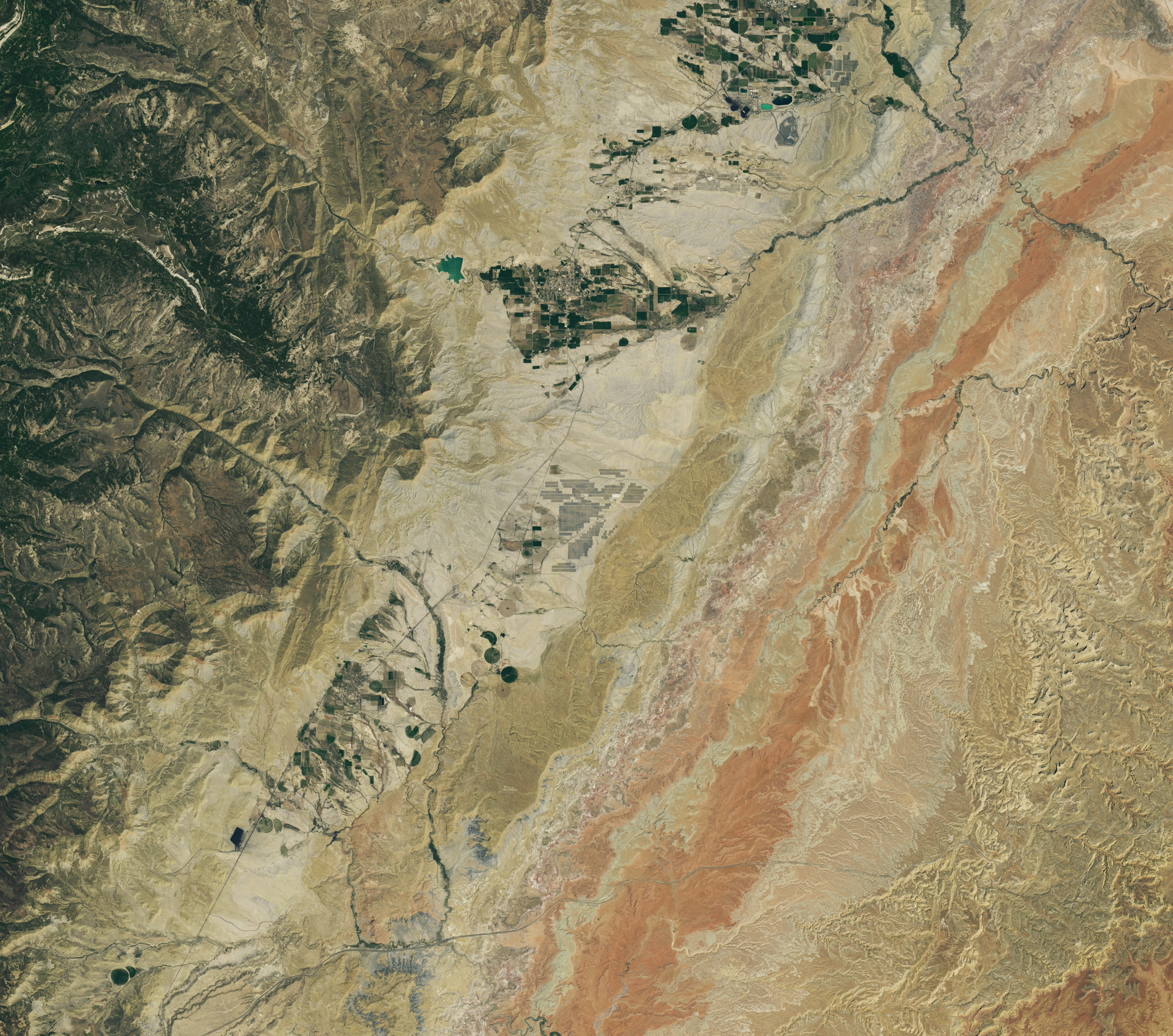
Grid-like arrays of solar panels cover parts of a valley floor in a brown, dry-looking area of Utah.
NASA Earth Observatory / Lauren Dauphin
A dry, tan-colored valley containing a few circular irrigated fields runs roughly north-south through the image.
NASA Earth Observatory / Lauren Dauphin
Grid-like arrays of solar panels cover parts of a valley floor in a brown, dry-looking area of Utah.
NASA Earth Observatory / Lauren Dauphin
June 16, 2024
June 6, 2026
The nearly one million photovoltaic panels of a solar energy and battery storage facility in Utah appear in the right image, acquired with the OLI (Operational Land Imager) on Landsat 8 on June 6, 2026. The same sensor captured the left image on June 16, 2024. NASA Earth Observatory images by Lauren Dauphin.
Historically, central Utah’s Castle Valley has been a coal hub, with mining operations on the slopes of the Wasatch Plateau to the west active since the late 1800s. A different energy development arrived in the region in June 2026, when a large solar power and battery storage plant came online in the sunny valley about 130 miles (210 kilometers) southeast of Salt Lake City.
The recently constructed Green River Energy Center, seen in the Landsat 8 image above (right), features nearly one million solar panels and roughly 500 batteries on several square miles of previously undeveloped land. The facility has 400 megawatts of solar-generating capacity with another 400 megawatts of battery storage. That places it among the many utility-scale solar power and battery storage projects that the U.S. Energy Information Administration expects to be plugged into the country’s grid in 2026.
The Utah facility is slated to supply power to Salt Lake City and other areas across the state, according to news reports, and project staff estimate it could produce enough electricity for more than 100,000 homes. With its integrated battery storage, the plant has the potential to generate power at all hours, even when the Sun isn’t shining. And the Green River Energy Center can build on Castle Valley’s energy legacy by utilizing existing transmission lines originally built for coal-fired power plants in the area.
Though Utah adopted coal as its state rock and has long relied on it for energy, other sources, such as solar and geothermal, are becoming larger parts of the state’s energy mix. In 2025, coal fueled about half of the state’s electricity generation, down from about 75 percent in 2015. Meanwhile, solar grew to account for about 14 percent of generation in 2025, up from nearly zero a decade before. Satellite data can be useful to planners and policymakers involved in energy transitions for assessing the potential of renewable energy systems and tracking their adoption and performance.
NASA Earth Observatory images by Lauren Dauphin, using Landsat data from the U.S. Geological Survey. Story by Lindsey Doermann.
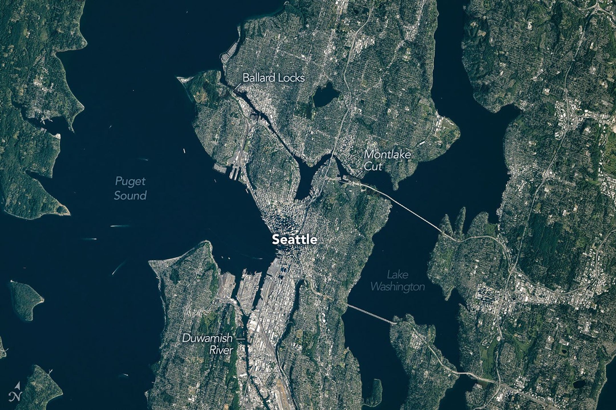
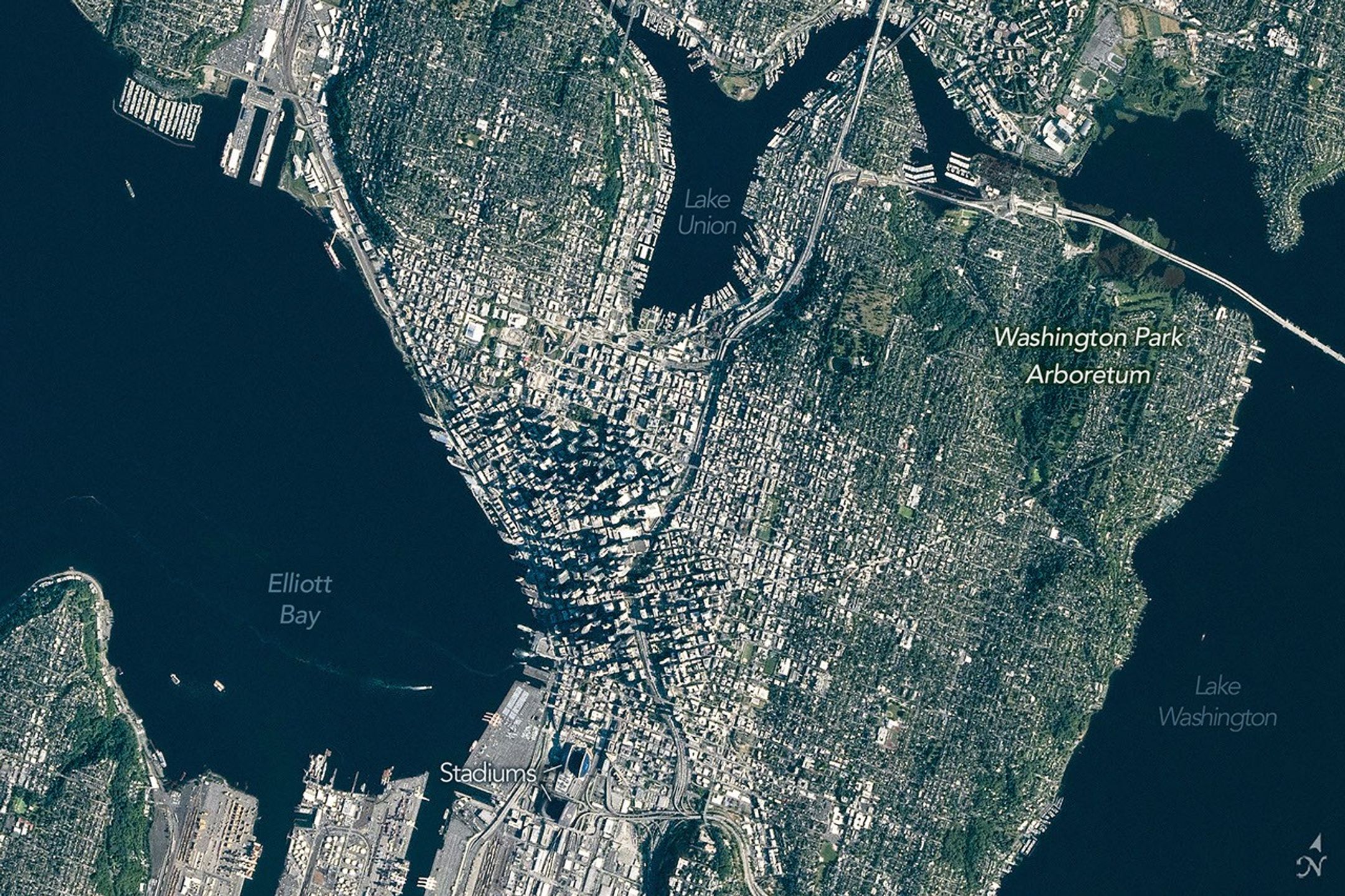
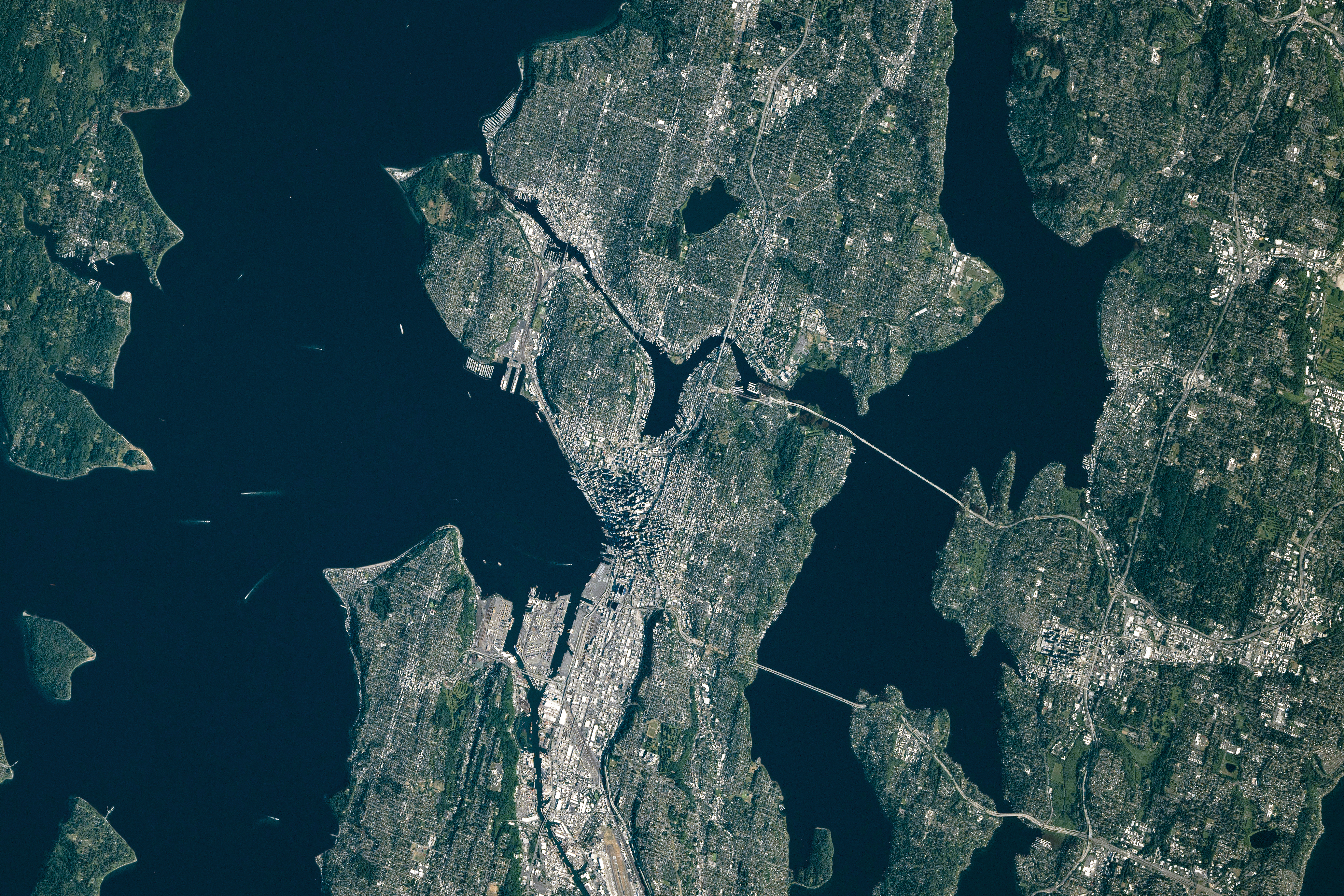
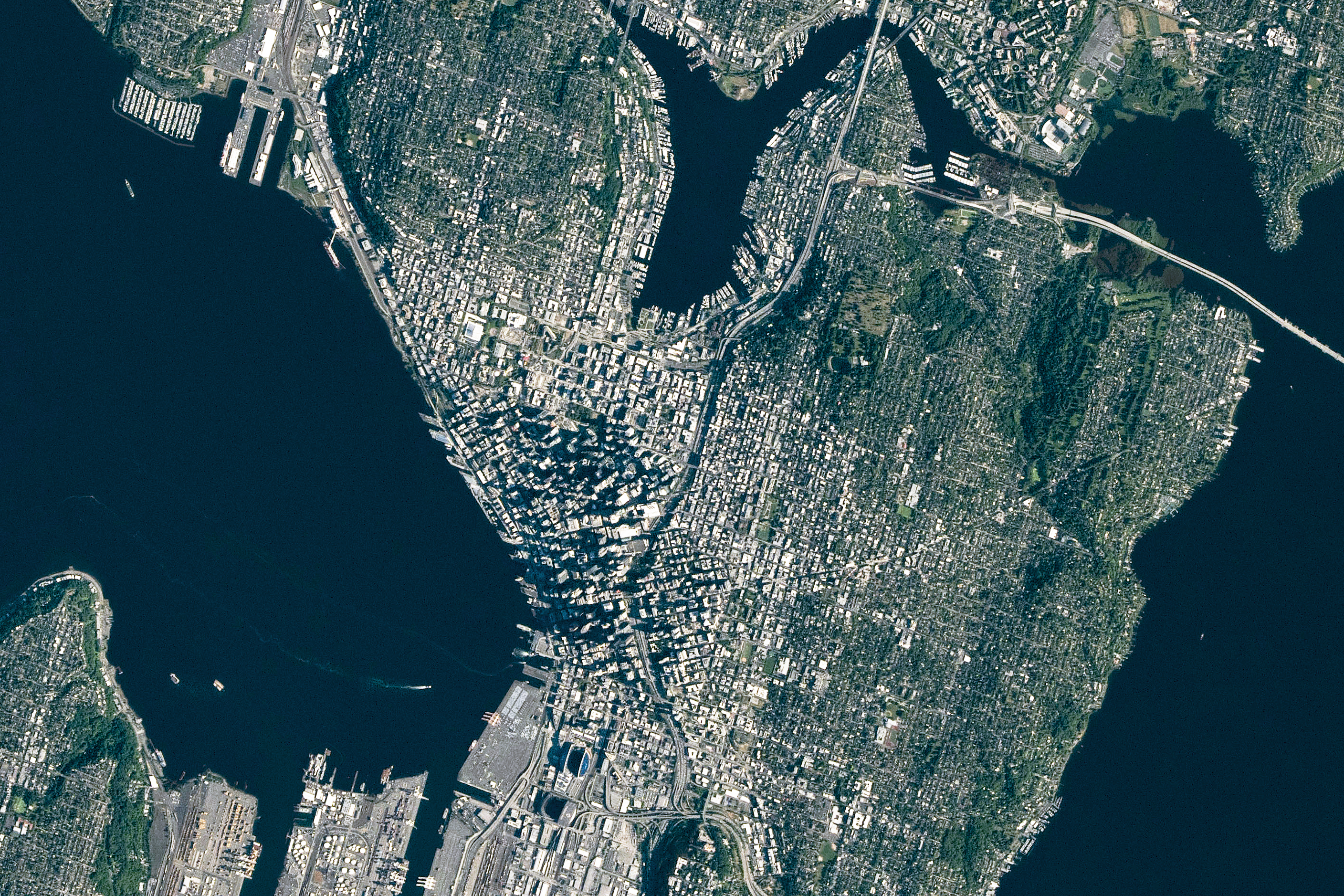
Seattle, Washington—sometimes known as the “Emerald City”—was glimmering in the morning sunlight when an astronaut aboard the International Space Station took this photo on June 16, 2026. The city’s parks and tree-filled neighborhoods lend a lush, green look to the metropolis, while tall buildings downtown cast long shadows and ships navigate surrounding waterways.
The broad contours of the city’s landscape and the water around it owe their shape to the advance and retreat of glaciers during the last ice age. Between roughly 18,000 and 16,000 years ago, the Puget lobe of the Cordilleran ice sheet covered the area in a mass of ice up to 3,300 feet (1,000 meters) thick. The glacier scoured the basins now occupied by Puget Sound and the region’s lakes.
The glacier left its mark above water, too. Several of Seattle’s notorious hills (of which there are seven or more, depending on who’s counting) are drumlins. These elongated mounds of glacial debris run north-south, parallel to the direction of the ice’s movement. East-west travelers in the city, facing challenging ups and downs, may attest to this topographic trend.
The ice also transported large boulders called glacial erratics from more northerly locations and deposited them around the region. A particularly large erratic, the Wedgwood Rock, stands about 20 feet (6 meters) tall and draws its name from the North Seattle neighborhood in which it rests.
June 16, 2026
In more recent times, humans have undertaken projects to rework the topography. Notable alterations include leveling Denny Hill north of downtown and filling in tideflats at the mouth of the Duwamish River south of downtown, which created around 1,300 acres of new land. Seattle’s professional sports stadiums sit atop this fill.
This photo was acquired after several development projects to update waterfront infrastructure downtown, initiated in 2010, were completed. These include a new ferry dock and terminal, a rebuilt seawall, and a tunnel to replace an above-ground highway and create more inviting public access to the waterfront.
Some replumbing of the region’s waterways is apparent from the astronaut’s perspective, as well. In the 1910s, the Army Corps of Engineers built canals on either side of Lake Union to connect Puget Sound (an inlet of the Pacific Ocean) with Lake Washington. Starting in 1916, the Montlake Cut connected Lake Washington to Lake Union, and the Ballard Locks, northwest of Lake Union, began raising and lowering watercraft between the freshwater lakes and tidal Puget Sound. As a result of this project, Lake Washington’s water level dropped about 9 feet (3 meters) and ceased draining from its natural outlet at its southern end.
Today, the waters in and around Seattle support many uses: container ships, cruise ships, car and passenger ferries, floatplanes, and recreational craft ply the sound and lakes. And as for Seattle’s emerald nickname, pockets of old-growth forest still exist within city limits, containing centuries-old trees such as Douglas fir, Western red cedar, and Western hemlock. Seattleites often spot wildlife such as bald eagles, coyotes, and sea lions in the city’s various habitats.
Astronaut photograph ISS074-E-723719 was acquired on June 16, 2026, with a Nikon Z9 digital camera using a focal length of 560 millimeters. It is provided by the ISS Crew Earth Observations Facility and the Earth Science and Remote Sensing Unit at NASA Johnson Space Center. The image was taken by a member of the Expedition 74 crew. The image has been cropped and enhanced to improve contrast, and lens artifacts have been removed. The International Space Station Program supports the laboratory as part of the ISS National Lab to help astronauts take pictures of Earth that will be of the greatest value to scientists and the public, and to make those images freely available on the Internet. Additional images taken by astronauts and cosmonauts can be viewed at the NASA/JSC Gateway to Astronaut Photography of Earth. Story by Lindsey Doermann.
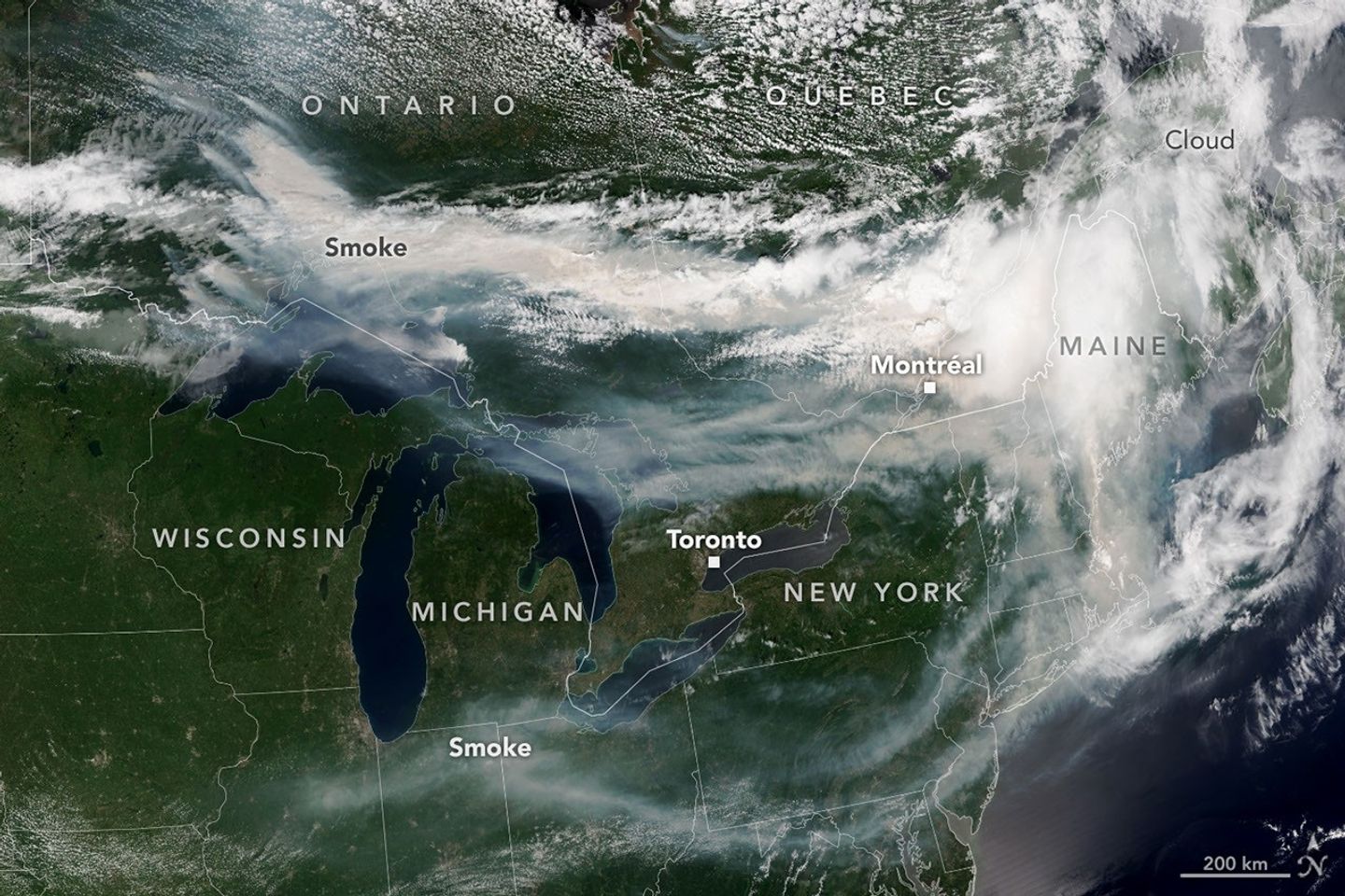
Smoke from wildland fires pours eastward over Canada and the U.S. in an image captured on the afternoon of July 14, 2026, by the VIIRS (Visible Infrared Imaging Radiometer Suite) on the NOAA-21 satellite.
NASA Earth Observatory/Lauren Dauphin
After a slow start to Canada’s 2026 fire season, activity picked up by the end of June amid dry, warm conditions and returned closer to the 25-year average. By mid-July, almost 850 fires were actively burning across the country, according to the Canadian Interagency Forest Fire Centre. More than 180 of those were burning in Ontario.
This NOAA-21 image, acquired on the afternoon of July 14, 2026, shows smoke billowing from the Ontario fires. Winds carried the smoke primarily southeast over much of the southern part of the province, as well as parts of Quebec and the U.S. Midwest and Northeast, tinting the sky shades of gray and yellow and the Sun orange in many areas.
The smoke’s impact on air quality varied, depending largely on altitude. In areas where smoke was high in the atmosphere, air quality impacts were negligible; where it drifted closer to the ground, conditions worsened. Air quality in Toronto, for instance, reached unhealthy levels, according to AirNow. People in the southern parts of the province were also grappling with a heat wave, compounding the health risks.
Much of the smoke came from fires in Northwestern Ontario, where eight blazes saw significant growth on July 13 and 14. The fires prompted officials to issue evacuation orders for several communities in this part of the province, according to news reports.
As of July 14, fires across Canada have burned 1.9 million hectares (4.7 million acres) since the start of the year—still well below the season totals from the extreme fire years of 2023 and 2025. How the rest of the season plays out remains to be seen. A seasonal fire outlook—compiled by wildland fire experts from the U.S., Canada, and Mexico—shows where fire conditions are more or less likely through July, August, and September.
NASA Earth Observatory image by Lauren Dauphin, using VIIRS data from NASA EOSDIS LANCE , GIBS/Worldview , and the Joint Polar Satellite System (JPSS). Story by Kathryn Hansen.
Downloads
July 14, 2026
JPEG (3.96 MB)
References & Resources
AirNow (2026, July 15) Wildfires. Accessed July 15, 2026.
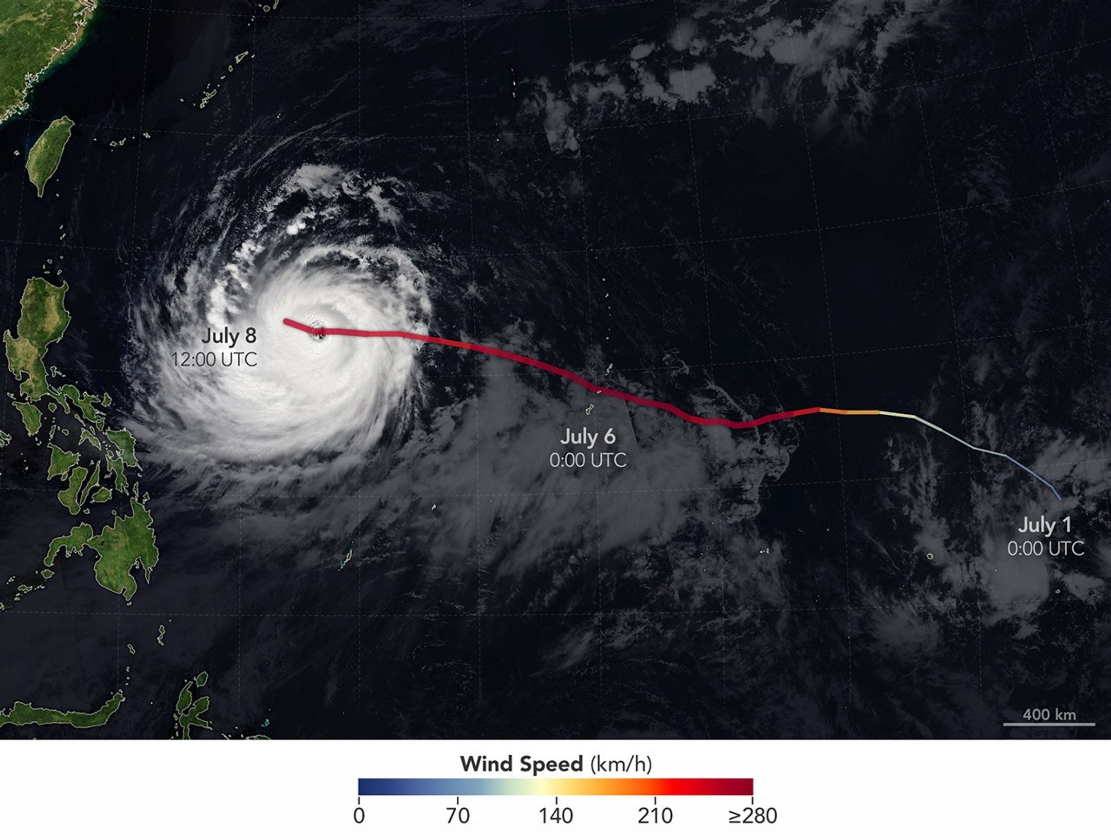
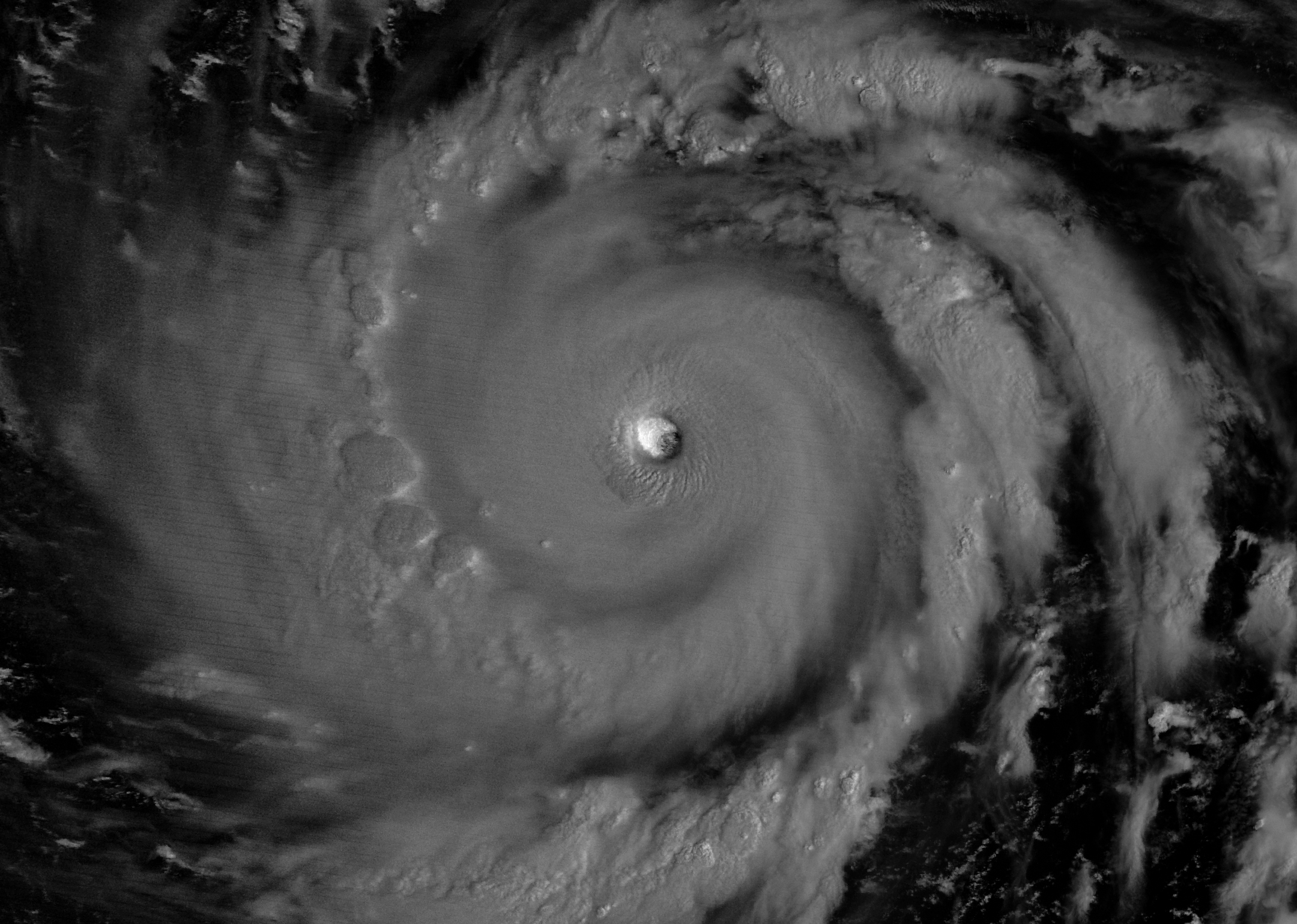
Moonlight illuminates the western side of Super Typhoon Bavi’s eyewall at about 15:30 Universal Time on July 5 (1:30 a.m. local time on July 6). The image was acquired with the VIIRS (Visible Infrared Imaging Radiometer Suite) day-night band on the NOAA-20 satellite.
NASA Earth Observatory/Michala Garrison
In early July 2026, for the second time in three months, a powerful typhoon crossed the U.S. Northern Mariana Islands and Guam in the North Pacific Ocean. Super Typhoon Bavi was at peak intensity when it neared the islands on the night of July 5, bringing winds of 290 kilometers (180 miles) per hour, along with torrential rain and dangerous storm surge.
This nighttime image, captured by the VIIRS (Visible Infrared Imaging Radiometer Suite) on the NOAA-20 satellite, shows Bavi’s eye at about 15:30 Universal Time on July 5 (1:30 a.m. local time on July 6). Light from the Moon, which was in the waning gibbous phase, illuminates the eyewall’s western side. The eye passed over Rota, north of Guam, several hours after the image was acquired.
Bavi became a super typhoon in the early hours of July 4 local time while tracking west over the warm ocean. Satellite observations indicated that sea surface temperatures were around 30 degrees Celsius (86 degrees Fahrenheit) in the region. Bavi was the third tropical cyclone in 2026 to reach category 5 intensity on the Saffir-Simpson wind scale.
The typhoon caused extensive damage across Guam, Rota, and Saipan, according to news reports, downing power poles and lines; flooding roads and littering them with debris; and damaging buildings, including a water distribution station on Rota. U.S. Coast Guard crews worked to clear navigation hazards in the waterways around Guam and the Northern Marianas and reopen ports as dangerous marine conditions subsided, according to reports. This damage comes on top of destructive winds and flooding from Super Typhoon Sinlaku, which crossed the islands in mid-April.
Super Typhoon Bavi tracked west over the Northern Mariana Islands toward Asia in early July 2026. The storm’s clouds and path are overlaid on a Blue Marble: Next Generation image built from scenes captured by the MODIS (Moderate Resolution Imaging Spectroradiometer). The image of the storm was captured by the VIIRS (Visible Infrared Imaging Radiometer Suite) on the NOAA-21 satellite on July 8, 2026, at about 04:30 Universal Time.
NASA Earth Observatory/Michala Garrison
On July 8, Bavi remained a powerful typhoon as it moved west over the Philippine Sea. In the early afternoon, when the image above was captured, the National Weather Service reported maximum sustained wind speeds of 250 kilometers (155 miles) per hour. Forecasts indicated the typhoon’s track could bend northwest toward Taiwan, the Ryukyu Islands of southern Japan, and mainland China and weaken over the next several days.
Writing in Yale Climate Connections, meteorologist Jeff Masters said that Bavi is the type of storm that might be expected when a strong El Niño event is building, which is currently the case. El Niño-year typhoons may form farther east, giving them more time over warm water to intensify before curving toward Asia, Masters explained, “resulting in a greater chance of reaching Category 5 intensity.”
Mountainous landscapes appear green and untouched by fire in a satellite image acquired on June 5, 2026.
NASA Earth Observatory/Michala Garrison
An image of the same area shows a large brown patch spanning much of the image in an image acquired after the fire on June 29, 2026.
NASA Earth Observatory/Michala Garrison
June 5
June 29
A burned landscape spans more than 150 square miles (390 square kilometers) of rugged terrain northwest of Junction, Utah, as seen in this pair of images captured by the OLI (Operational Land Imager) on Landsat 8 and Landsat 9 on June 5, 2026 (left) and June 29, 2026 (right). NASA Earth Observatory images by Michala Garrison.
After a winter of below-average snowpack and an unusually warm and dry start to summer, the National Interagency Fire Center warned that the Great Basin and parts of the Rockies faced an elevated risk of wildfires in July 2026.
The warning proved accurate. By July 7, firefighters labored to contain nearly three dozen large, early-season wildland fires that raced through forests in several parts of the western U.S. Utah was among the most active states, with fires having charred 558 square miles (1,445 square kilometers) and four major fires that were not fully contained still burning.
The Cottonwood fire ranked as one of Utah’s—and the country’s—largest and most destructive fires of the year so far. As of July 7, it had burned 150 square miles (390 square kilometers), just shy of the Babylon fire in eastern Utah. Landsat 9 captured the false-color image (bands 7-5-4) above (right) on June 29, 2026, when blackened vegetation spanned a large patch of rugged terrain along the Beaver River. The image on the left shows the same area on June 5, a few weeks before the fire ignited. In this band combination of shortwave infrared, near infrared, and visible light, unburned vegetation appears bright green, snow is blue, and clouds are white.
Ponderosa pine, oak, sagebrush, and grasses were among the vegetation types that burned. Officials with the state’s forestry division told news media that the Cottonwood fire had destroyed up to 150 structures. Eagle Point Ski Resort, which lost more than 100 condos and 30 cabins, also reported damage to four of its five chairlifts.
The damage to forests was extensive, though isolated patches survived largely unscathed, remaining as green oases within the broader burned area. Among them were the forests around Tushar Campground, the site of a 4-H summer camp. Beaver County officials credited years of forest treatments, such as clearing brush and trimming branches, with helping save the campground and surrounding forests.
The fire spreads especially rapidly on June 23 and June 26. The fire perimeters in this visualization are based on data from NASA’s Fire Events Data Suite.
NASA Earth Observatory/Michala Garrison
As the fire spread, NASA’s Fire Events Data Suite (FEDS) tracked its progression and rate of growth. The visualization above, based on the FEDS system, shows the fire surging on June 23 and tripling in size over 12 hours that day as it spread to the north, east, and south. It also grew rapidly on June 26, when it made a run to the north. FEDS draws on data from the VIIRS (Visible Infrared Imaging Radiometer Suite) sensors aboard the Suomi NPP, NOAA-20, and NOAA-21 satellites, which detect active fires day and night by their thermal infrared signature.
FEDS is one of several tools available to firefighters and emergency management officials when responding to fires. First responders often rely on higher-resolution airborne imagers or on firefighters walking fire edges to map perimeters. FEDS offers a different advantage: consistent, easily accessible data that do not need to be specially requested, according to Tempest McCabe, a University of Maryland scientist based at NASA’s Goddard Space Flight Center who helped develop the tool. As a result, FEDS often detects a fire’s start earlier than other sources and tracks blazes for their full duration. To capitalize on strengths like these, the FEDS team is working closely with operational fire behavior analysts, with support from NASA’s FireSense program, to better understand and anticipate periods of rapid fire spread.
A total of 1,289 firefighters have been deployed to the Cottonwood fire, according to InciWeb, a website managed by the National Interagency Fire Center. As of July 7, the fire was 56 percent contained, but forecasters expect a hot, dry weather pattern to persist in the coming days, with fire behavior likely to be “very active to extreme” over the next 72 hours.
Government satellite data are part of a global system of observations used to track fire behavior and analyze emerging trends. Among the real-time wildfire monitoring tools that NASA makes available are FIRMS (Fire Information for Resource Management System), the Worldview browser, and the Fire Event Explorer.
As of July 7, 2026, fires had burned 5,265 square miles (13,636 square kilometers) across the United States, according to the National Interagency Fire Center. That’s 46 percent more than the 10-year average (2016-2025) for that point in the season.
NASA Earth Observatory images by Michala Garrison, using Landsat data from the U.S. Geological Survey and fire perimeter data from the Fire Events Data Suite. Story by Adam Voiland.
Every month, NASA Earth Observatory features a puzzling satellite image. The July 2026 puzzler appears above.
Your Challenge Identify the location shown in this satellite image. Share what clues you see, where you think it is, and what makes this place interesting or unique to you.
How to Answer Submit your response using this form and select “Puzzler Answer” as the topic. Please include your preferred name or alias.
You can keep it simple and just guess the location. Want to impress us? Tell us which satellite and instrument captured the image, which spectral bands were used, or point out a subtle detail about the geology or history of the area. If something catches your eye, or if this is your home or means something to you, we’d love to hear about it.
The Prize We can’t offer prize money or a trip to space to see Earth like satellites and astronauts do. But we can offer something almost as rewarding: puzzler bragging rights.
About a week after the challenge, we’ll post the answer at the top of this page, along with a link to an Earth Observatory Image of the Day story that explains the image in more detail. We’ll recognize the first person who correctly guesses the location, and we may also highlight readers who share especially thoughtful or interesting answers. By submitting a response, you acknowledge that your comments may be edited, excerpted, and published on this page.
Until then, zoom in, look closely, and enjoy the challenge. See you at the reveal!
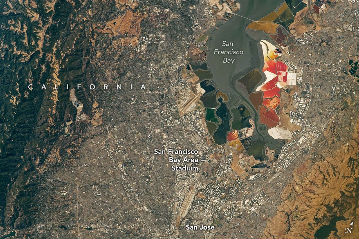
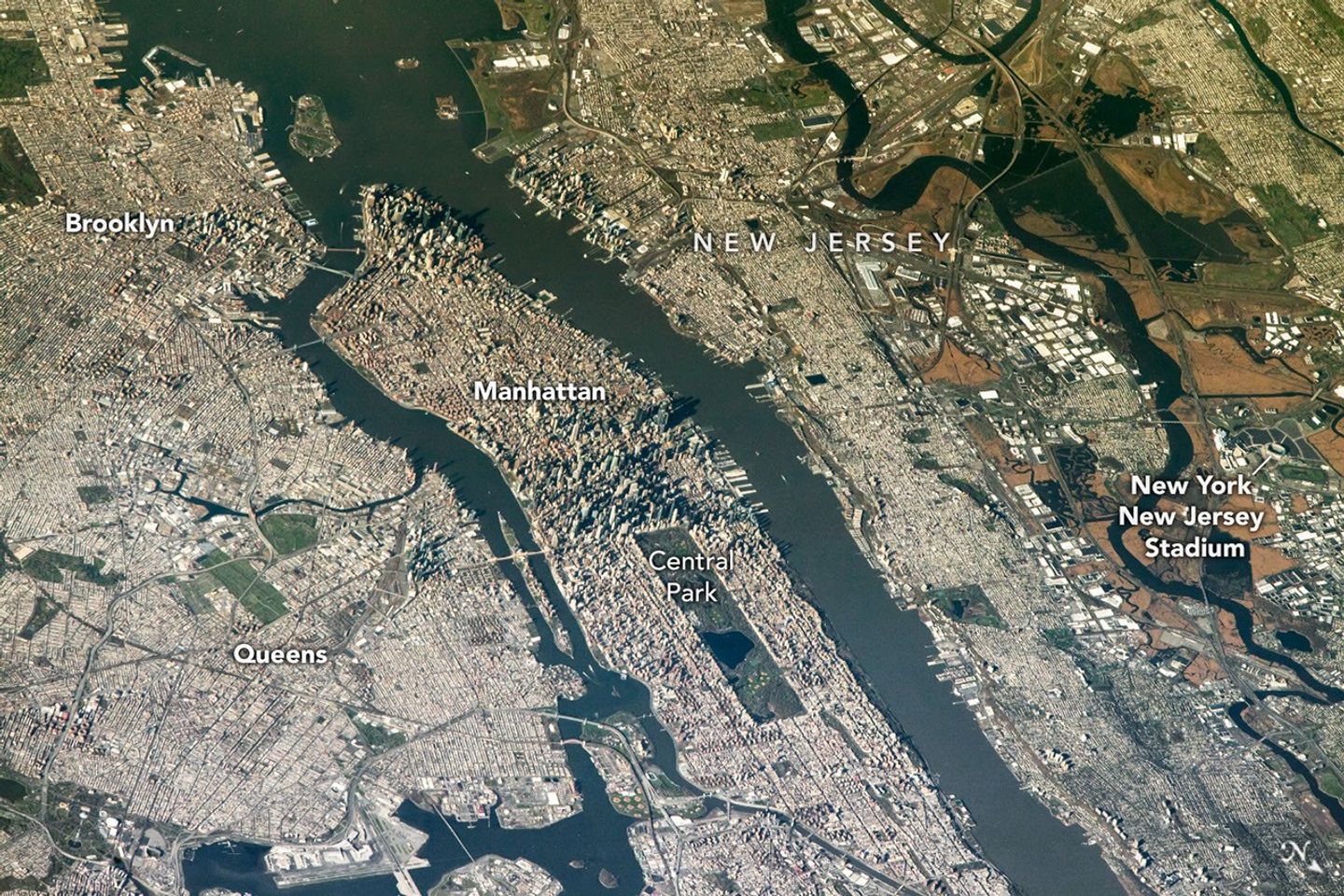
In summer 2026, sixteen stadiums across North America hosted matches as part of the FIFA World Cup. Over the years, astronauts aboard the International Space Station have captured a top-down view of the infrastructure, landscapes, and ecosystems surrounding many of these venues.
Six of the matches were played at the San Francisco Bay Area Stadium, beginning on June 13 with a match-up between Qatar and Switzerland. This stadium (also called Levi’s Stadium) is located in Santa Clara, California, adjacent to San Jose and around 40 miles (64 kilometers) south of San Francisco. An astronaut aboard the International Space Station took this photo (above) on July 26, 2022.
The stadium, completed in 2014, is surrounded by a mix of recreational, housing, and business infrastructure. The scene includes the southern part of San Francisco Bay, which is 23 years into a 50-year effort to restore up to 90 percent of the region’s salt ponds to tidal wetlands and marshlands, while retaining some of its salt-making heritage.
The Bay Area hosted its sixth and final World Cup match on July 1, when the U.S. faced off against Bosnia and Herzegovina in a knockout match. The U.S. advanced to the round of 16 following a 2-0 win.
April 17, 2022
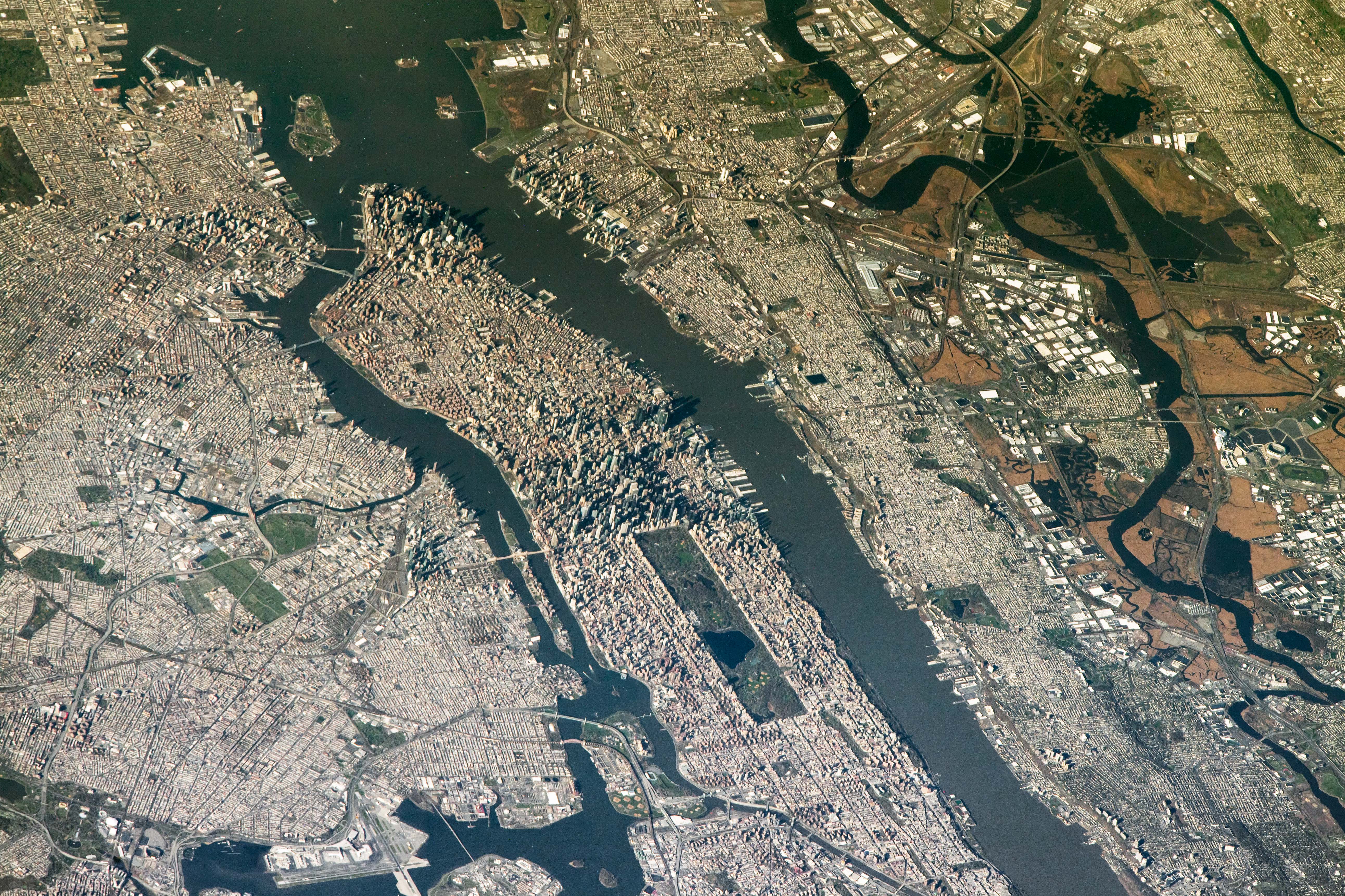
The FIFA World Cup final is scheduled for July 19 at New York New Jersey Stadium, part of the Meadowlands Sports Complex, in East Rutherford, New Jersey. The stadium (also called MetLife Stadium) sits along the New Jersey Turnpike, west of Midtown Manhattan. Note that north is toward the bottom-right of this photo, captured by an astronaut on April 17, 2022.
The area has seen centuries of human impact. Colonists cleared wetlands and cedar forest for settlements, and development for a range of economic and industrial uses followed. In the 20th century, it became an unregulated dumping ground. In recent decades, though, wetland restoration efforts have occurred alongside the development of the sports and entertainment complex.
Other World Cup host cities have also appeared in astronaut photography and satellite imagery. Guadalajara Stadium (Estadio Akron), Los Angeles Stadium (SoFi Stadium), Houston Stadium (NRG Stadium/Reliant Stadium), and BC Place Vancouver (BC Place) are among the venues that have been observed from above.
Astronaut photograph ISS067-E-202213 was acquired on July 26, 2022, with a Nikon D5 digital camera using a focal length of 400 millimeters, and astronaut photograph ISS067-E-18580 was acquired on April 17, 2022, with a Nikon D5 digital camera using a focal length of 1150 millimeters. They are provided by the ISS Crew Earth Observations Facility and the Earth Science and Remote Sensing Unit at NASA Johnson Space Center. The images were taken by a member of the Expedition 67 crew. The images have been cropped and enhanced to improve contrast, and lens artifacts have been removed. The International Space Station Program supports the laboratory as part of the ISS National Lab to help astronauts take pictures of Earth that will be of the greatest value to scientists and the public, and to make those images freely available on the Internet. Additional images taken by astronauts and cosmonauts can be viewed at the NASA/JSC Gateway to Astronaut Photography of Earth. Story by Kathryn Hansen.
In preparing to visit the Moon’s surface, soon-to-be lunar explorers in NASA’s Apollo program first ventured into a variety of unfamiliar landscapes on Earth. A couple of these trips, in the summers of 1965 and 1966, took astronauts to Alaska’s remote Katmai National Park for simulations of field geology in Moon-like environments.
In one exercise, which they called “playing the Moon game,” pairs of astronauts were placed at unfamiliar field sites and asked to pretend as if they were on the Moon. By the account of William Phinney, Apollo’s science training coordinator, they were tasked with collecting representative geologic samples and practicing how to communicate their observations to scientists.
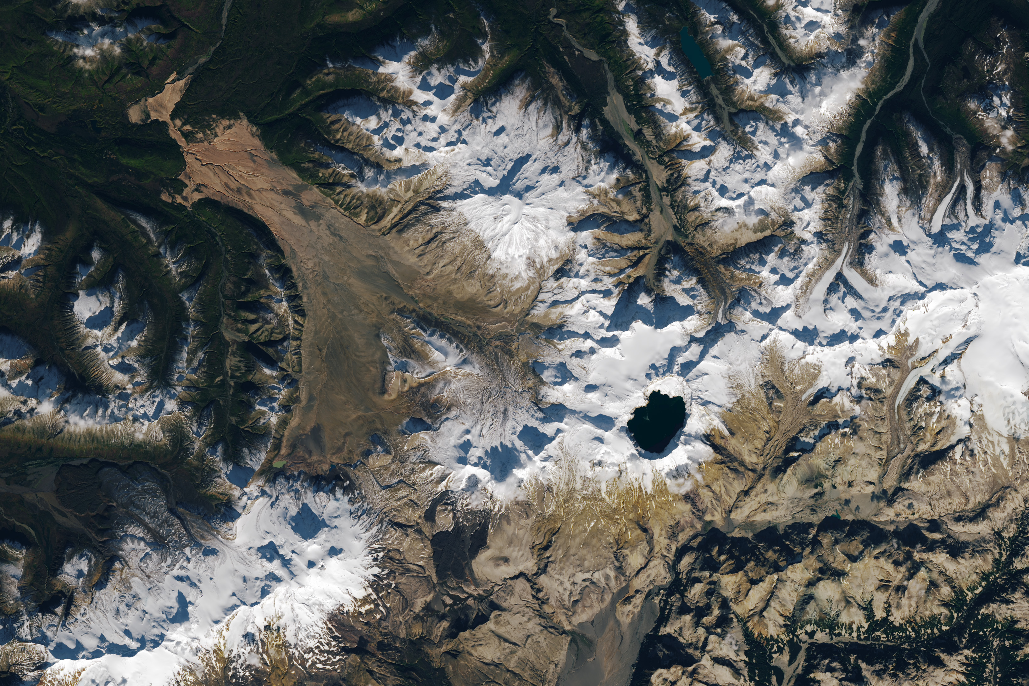
September 29, 2025
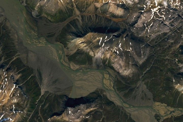
The Alaskan setting for the Moon game was an unusual volcanic landscape called the Valley of Ten Thousand Smokes. The valley is full of debris deposited by the 1912 eruption of Novarupta—the largest volcanic event on Earth in the 20th century.
The images above, acquired on September 29, 2025, with the OLI (Operational Land Imager) on Landsat 9, show the massive ash flow deposited by Novarupta. The layer measures up to 660 feet (200 meters) thick and was emplaced at a searing 1,380 degrees Fahrenheit (750 degrees Celsius).
The Valley of Ten Thousand Smokes, shown in the 1917 photo below, is so named because of the abundance of fumaroles—gas and steam-emitting vents—that filled the valley for a decade after the eruption. A few hundred persisted more than 10 years, with some lasting until the 1990s.
1917
Scientists initially suspected that the monster eruption occurred at Mount Katmai, a neighboring volcano with a large caldera located 6 miles (10 kilometers) east of Novarupta’s dome. However, they later determined that the eruption actually occurred at Novarupta—whose name means “new eruption”—after stealing magma from beneath Katmai. As the magma chamber emptied, Katmai collapsed, forming the 2.5-mile-wide (4-kilometer-wide) caldera present today.
The volcanic landscape in the Valley of Ten Thousand Smokes is far fresher than the ancient lava flows that formed the Moon’s volcanic features. But for the Apollo astronauts, it offered an “excellent opportunity to view volcanic materials and landforms in nearly pristine condition,” Phinney wrote. They studied evidence of fumaroles and examined vertical sections of the deposits where streams had eroded deep gorges.
June 9, 1991
Researchers continue to visit this Alaskan wilderness in search of clues that could help decipher the geology of the Moon and Mars. In 2024, the Goddard Instrument Field Team (GIFT) trekked to the Valley of Ten Thousand Smokes to study its icy volcanic landscape. Like the valley, Mars contains glaciers and ice sheets layered with dust and ash, a dynamic and difficult-to-interpret environment.
Advancing lunar science, the GIFT team also collected samples from rock formations comparable to the Moon’s Gruithuisen Domes. These mysterious features are made of hardened lava with a different composition than the surrounding rock. With more to learn about our nearest celestial neighbor, the spirit of the Moon game lives on in the 21st century.
NASA Earth Observatory images by Lauren Dauphin, using Landsat data from the U.S. Geological Survey. Photos from National Geographic Society Katmai expeditions photographs, Archives and Special Collections, Consortium Library, University of Alaska Anchorage, and from the U.S. Geological Survey Volcano Hazards Program. Story by Lindsey Doermann.
From Civil War battlegrounds to industrial landmarks to the country’s earliest national parks, these places helped shape the United States we know today.
Samuel Pierpont Langley conducted the first successful flight of an unpiloted, engine-driven, heavier-than-air craft from a houseboat near Chopawamsic Island…
Tropical Storm Arthur’s white storm clouds cover the waters off the U.S. Gulf Coast. Some clouds extend inland over parts of Texas and Louisiana.
NASA Earth Observatory/Michala Garrison
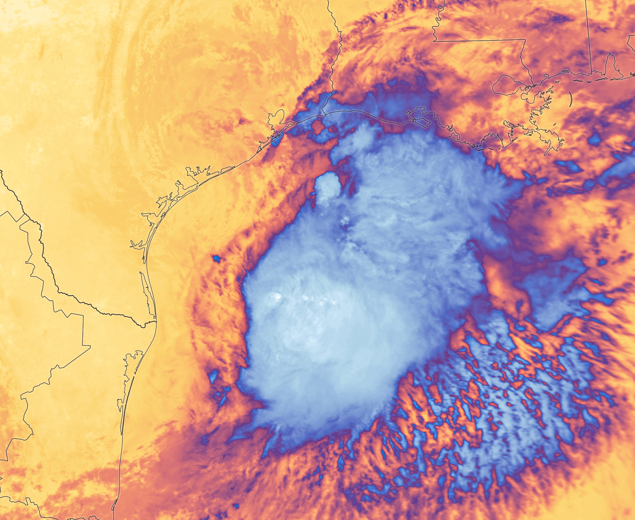
White and purple areas of cloud off the Gulf Coast indicate the cooler areas of cloud tops associated with Tropical Storm Arthur.
NASA Earth Observatory/Michala Garrison
Natural color
brightness temperature
Images from the MODIS (Moderate Resolution Imaging Spectroradiometer) on NASA’s Terra satellite show Tropical Storm Arthur on the morning of June 17, 2026. The left image is natural color; the right shows infrared signals known as brightness temperature. NASA Earth Observatory images by Michala Garrison.
Tropical Storm Arthur, the first named storm of the 2026 Atlantic hurricane season, brought high winds and heavy rain to the U.S. Gulf Coast in mid-June.
NASA’s Terra satellite captured this natural-color image (left) at 10:30 a.m. Central Time (15:30 Universal Time) on June 17. The second image (right) depicts infrared signals known as brightness temperature, which help distinguish cooler cloud tops (white and purple) from the warmer surface below (yellow and orange). Around the time these images were acquired, the system had just recently been designated a tropical storm, according to the National Hurricane Center (NHC).
Though Arthur stayed below hurricane strength, it still delivered strong winds to parts of the Gulf Coast as it tracked northeast. The storm had maximum sustained winds of 40 miles (65 kilometers) per hour around the time these images were captured. Tropical-storm-force winds extended 175 miles (280 kilometers) from the storm’s center, the NHC reported. Measurements at Galveston, Texas, for instance, showed a gust of 48 miles per hour.
The storm also produced heavy rainfall that the National Weather Service warned could lead to life-threatening flash flooding. Estimates from IMERG (the Integrated Multi-Satellite Retrievals for GPM), a product of the GPM (Global Precipitation Measurement) mission, showed high rainfall rates over Gulf waters and extending inland on June 17.
As Arthur weakened and became less organized, it continued to bring abundant moisture to central Gulf Coast states on June 18. The National Weather Service reported rainfall rates of 3 inches (7.6 centimeters) per hour in southeastern Louisiana. Forecasts indicated that storm-total rainfall amounts could exceed 12 inches (30 centimeters) in areas, with some locations seeing totals approaching 20 inches (51 centimeters).
NASA Earth Observatory images by Michala Garrison, using MODIS data from NASA EOSDIS LANCE and GIBS/Worldview. Story by Kathryn Hansen.
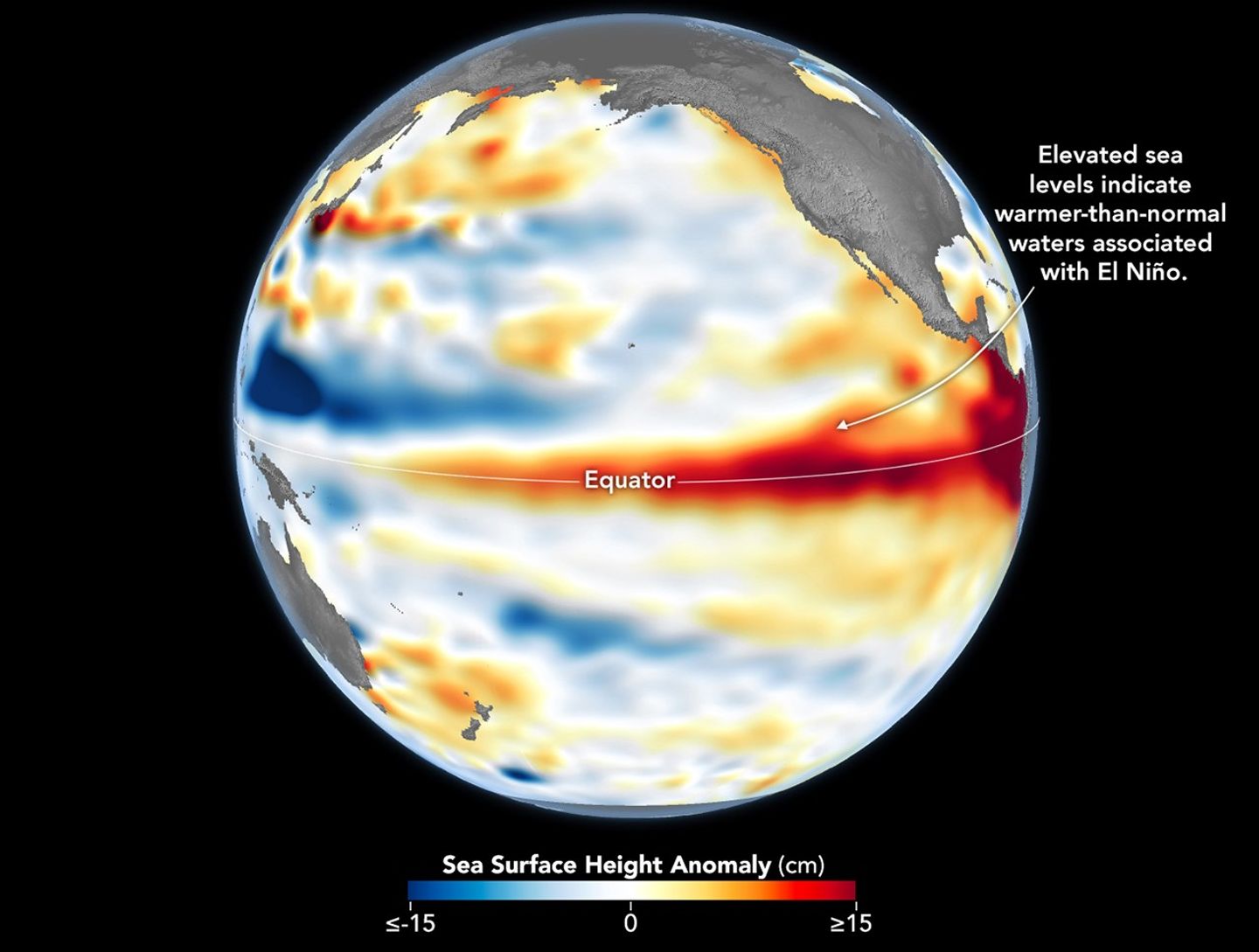
Higher-than-normal sea surfaces (red) are visible in the central and eastern Pacific on June 8, 2026, a few days before El Niño was declared. Data for the map were acquired by the Sentinel-6 Michael Freilich satellite and processed by scientists at NASA’s Jet Propulsion Laboratory (JPL).
NASA Earth Observatory/Lauren Dauphin
El Niño, characterized by warmer-than-normal water temperatures in parts of the equatorial Pacific, made its return in June 2026. Observations of sea surface height from the Sentinel-6 Michael Freilich satellite that month indicated that the 2026 event was continuing to strengthen.
The natural, recurring phenomenon can have widespread effects, typically bringing wetter conditions to the U.S. Southwest and drought to countries in the western Pacific, such as Indonesia and Australia. NOAA declared an El Niño on June 11, after sea surface temperatures in the central and eastern equatorial Pacific measured at least 0.5 degrees Celsius above average for several consecutive months.
Meanwhile, NASA scientists have been observing a complementary sign of El Niño: areas of elevated sea surface height. When ocean water warms, it expands in volume and causes the sea surface to rise—making the water’s height a reliable indicator of ocean temperatures. Warmer-than-normal temperatures, hence higher sea surface heights, in parts of the equatorial Pacific Ocean are associated with El Niño.
The map above depicts sea surface height anomalies across the central and eastern Pacific Ocean as observed on June 8, 2026. Shades of red indicate sea levels that were higher than average. Normal sea level conditions appear white, and lower areas are blue.
Data for the map were acquired by the Sentinel-6 Michael Freilich satellite—launched in 2020 by NASA and led by ESA (European Space Agency)—and processed by scientists at NASA’s Jet Propulsion Laboratory (JPL). Note that signals related to seasonal cycles and long-term trends have been removed to highlight sea level anomalies associated with El Niño and other short-term natural phenomena.
Earlier in spring 2026, the satellite started to detect precursor signs of El Niño as swells of warm water hundreds of miles wide, known as Kelvin waves, moved from the western Pacific to the eastern Pacific. That happens when trade winds in the western equatorial Pacific weaken and then temporarily reverse to blow from the west. Warm water piles up in the east, deepening the warm surface layer, lowering the thermocline, and suppressing the upwelling that usually keeps waters along the Pacific coasts of the Americas cooler.
This buildup of heat beneath the water’s surface is what sea surface height observations capture. It goes beyond surface temperature measurements to indicate how much heat is stored in the subsurface. That’s important because a shallow warm layer might not have much impact on climate and weather, while a large reservoir of heat below the surface can matter more.
According to JPL sea level researcher Severine Fournier, deputy project scientist for Sentinel-6 Michael Freilich, conditions in the western Pacific on June 8 looked similar to those from the same time in 1997, a year when an exceptionally strong El Niño emerged. Warm conditions in the eastern Pacific in 2026 have lagged behind, however, with fewer Kelvin waves built up by the same date.
Still, more warm Kelvin waves appeared to be approaching the eastern Pacific, meaning El Niño was still strengthening. Whether it catches up to 1997 depends on ocean activity in the coming weeks. “For now, it looks like it’s going to be a big one—more so than I would have said last week—but we still need more observations to know what’s going to happen.”
NASA Earth Observatory image by Lauren Dauphin, using modified Copernicus Sentinel data (2023) processed by the European Space Agency and further processed by Josh Willis, Severin Fournier, and Kevin Marlis/NASA/JPL-Caltech. Story by Kathryn Hansen.
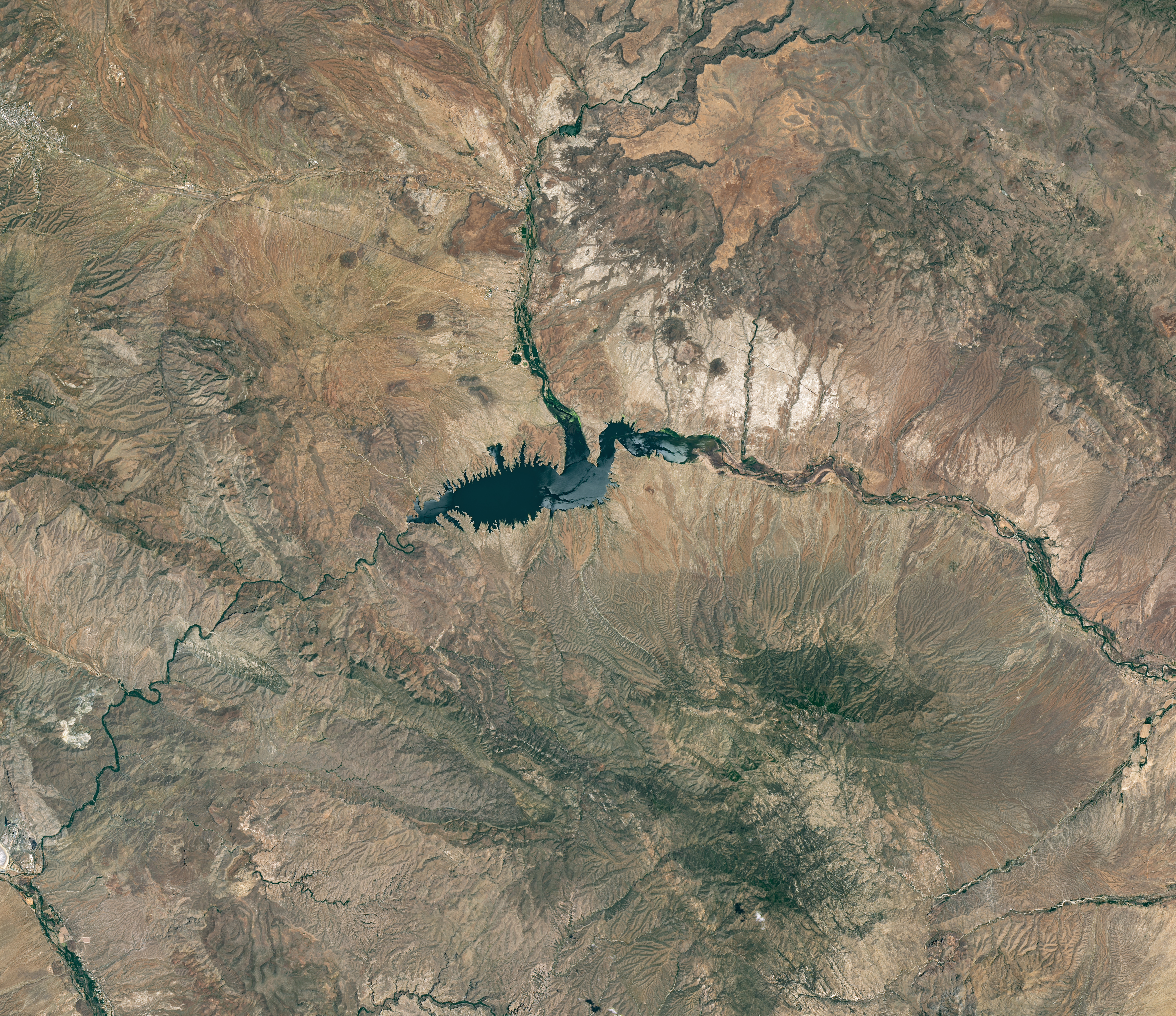
The reservoir appears lake-like and expansive in an image acquired in June 2023.
NASA Earth Observatory/Michala Garrison
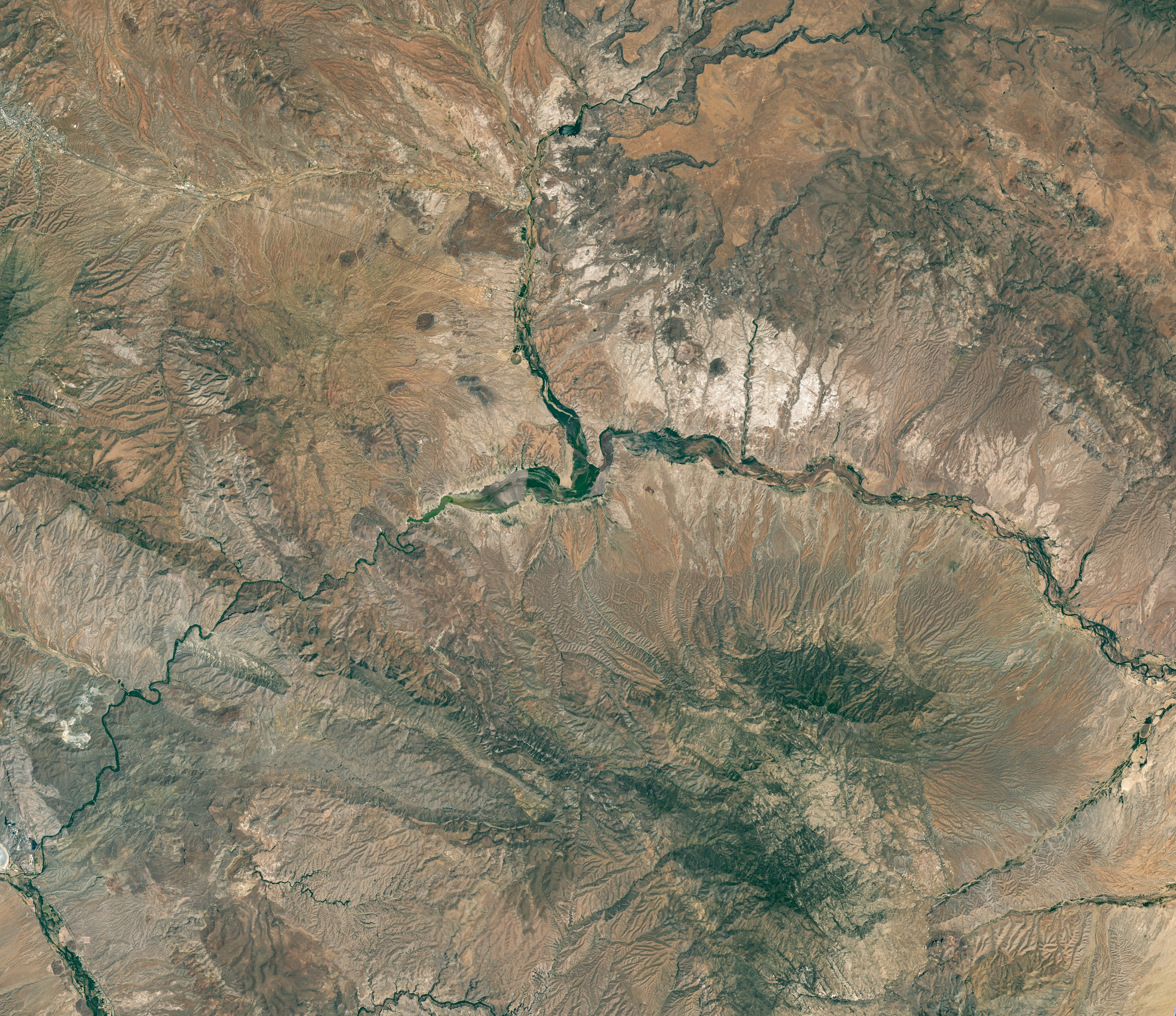
The reservoir is nearly empty by May 2026. The Gila River’s natural channel is now visible and flanked with green vegetation in what had been the bottom of the reservoir.
NASA Earth Observatory/Michala Garrison
June 7, 2023
May 22, 2026
Little water remains in the San Carlos Reservoir in May 2026 (right) compared to fuller conditions in June 2023 (left). Images were captured by the OLI (Operational Land Imager) on the Landsat 9 and 8 satellites, respectively. NASA Earth Observatory images by Michala Garrison.
The Gila River is among the Southwest’s most important rivers, delivering water for people, farms, and wildlife while linking the snow-fed mountains of southwestern New Mexico to the desert lowlands of southwestern Arizona.
In wetter years, seasonal snowfall on the Mogollon Mountains and Black Range provides much of the river’s spring flow and helps refill San Carlos Reservoir, which is formed by the Coolidge Dam. When filled to capacity, the reservoir is one of Arizona’s largest bodies of water.
However, in 2026, lackluster snowfall left the mountain snowpack in the Gila River watershed at 2 percent of the 1991-2020 March median. The limited snowpack pushed April streamflow to 39 percent of normal. By June, after mandatory water releases for downstream agriculture, the reservoir held less than 400 acre-feet of water.
The Landsat image above (right) shows the near-empty reservoir on May 22, 2026, when it stored 389 acre-feet of water—less than 1 percent full; the other image (left) shows the same area in June 2023, when it was about 60 percent full. The green vegetation growing along the river channel and reservoir edge includes a mixture of tamarisk, willow, cottonwood, sedges, and grasses.
Officials closed the reservoir indefinitely on June 5, 2026, after the declining water levels contributed to low oxygen levels—hypoxia—that killed virtually all of its fish. Species living in the reservoir included largemouth bass, black crappie, bluegill, channel catfish, flathead catfish, and several stocked species, including brown trout and rainbow trout. The decomposing fish may pose health risks to people attempting to boat or fish, the San Carlos Recreation and Wildlife Department warned.
The reservoir has hit similarly low water levels in the past, running out of water at least 20 times since it was filled in 1930, according to news reports. Even when the dam and reservoir were first dedicated, there was enough grass growing on the dried reservoir bottom that humorist Will Rogers famously quipped to President Calvin Coolidge: “If that was my lake, I’d mow it.”
Other years with major fish kills include 1976 and 2018. After more than 5 million fish died during a similar event in 1976, the Gila Heraldreported that it took five years for the lake’s ecosystem to rebound.
The region is currently in the midst of a multi-year dry period that has left much of the Gila River’s headwaters in New Mexico in a state of severe drought, according to data from the U.S. Drought Monitor.
However, the river’s flow is highly variable, and heavy rains during the coming wet season could help the reservoir recover. A seasonal monsoon outlook released by NOAA in May 2026 projected a 33 to 50 percent chance that an above-average amount of rain would fall in the region that summer. El Niño in the central and eastern equatorial Pacific, which was strengthening in late spring 2026, can make heavy rains in the U.S. Southwest more likely.
NASA Earth Observatory images by Michala Garrison, using Landsat data from the U.S. Geological Survey.Story by Adam Voiland.
The reservoir appears lake-like and expansive in an image acquired in June 2023.
NASA Earth Observatory/Michala Garrison
The reservoir is nearly empty by May 2026. The Gila River’s natural channel is now visible and flanked with green vegetation in what had been the bottom of the reservoir.
NASA Earth Observatory/Michala Garrison
June 7, 2023
May 22, 2026
Little water remains in the San Carlos Reservoir in May 2026 (right) compared to fuller conditions in June 2023 (left). Images were captured by the OLI (Operational Land Imager) on the Landsat 9 and 8 satellites, respectively. NASA Earth Observatory images by Michala Garrison.
The Gila River is among the Southwest’s most important rivers, delivering water for people, farms, and wildlife while linking the snow-fed mountains of southwestern New Mexico to the desert lowlands of southwestern Arizona.
In wetter years, seasonal snowfall on the Mogollon Mountains and Black Range provides much of the river’s spring flow and helps refill San Carlos Reservoir, which is formed by the Coolidge Dam. When filled to capacity, the reservoir is one of Arizona’s largest bodies of water.
However, in 2026, lackluster snowfall left the mountain snowpack in the Gila River watershed at 2 percent of the 1991-2020 March median. The limited snowpack pushed April streamflow to 39 percent of normal. By June, after mandatory water releases for downstream agriculture, the reservoir held less than 400 acre-feet of water.
The Landsat image above (right) shows the near-empty reservoir on May 22, 2026, when it stored 389 acre-feet of water—less than 1 percent full; the other image (left) shows the same area in June 2023, when it was about 60 percent full. The green vegetation growing along the river channel and reservoir edge includes a mixture of tamarisk, willow, cottonwood, sedges, and grasses.
Officials closed the reservoir indefinitely on June 5, 2026, after the declining water levels contributed to low oxygen levels—hypoxia—that killed virtually all of its fish. Species living in the reservoir included largemouth bass, black crappie, bluegill, channel catfish, flathead catfish, and several stocked species, including brown trout and rainbow trout. The decomposing fish may pose health risks to people attempting to boat or fish, the San Carlos Recreation and Wildlife Department warned.
The reservoir has hit similarly low water levels in the past, running out of water at least 20 times since it was filled in 1930, according to news reports. Even when the dam and reservoir were first dedicated, there was enough grass growing on the dried reservoir bottom that humorist Will Rogers famously quipped to President Calvin Coolidge: “If that was my lake, I’d mow it.”
Other years with major fish kills include 1976 and 2018. After more than 5 million fish died during a similar event in 1976, the Gila Heraldreported that it took five years for the lake’s ecosystem to rebound.
The region is currently in the midst of a multi-year dry period that has left much of the Gila River’s headwaters in New Mexico in a state of severe drought, according to data from the U.S. Drought Monitor.
However, the river’s flow is highly variable, and heavy rains during the coming wet season could help the reservoir recover. A seasonal monsoon outlook released by NOAA in May 2026 projected a 33 to 50 percent chance that an above-average amount of rain would fall in the region that summer. El Niño in the central and eastern equatorial Pacific, which was strengthening in late spring 2026, can make heavy rains in the U.S. Southwest more likely.
NASA Earth Observatory images by Michala Garrison, using Landsat data from the U.S. Geological Survey.Story by Adam Voiland.
The Nebraska Sandhills stretch across the north-central part of the state in this image acquired on August 19, 2025, with the OLI (Operational Land Imager) on Landsat 8.
NASA Earth Observatory/Lauren Dauphin
Editor’s Note: Today’s story is the answer to the June Puzzler.
The undulating landscape of north-central Nebraska may be easy to overlook among the iconic dune fields of the world. Far from any coast or desert, the Nebraska Sandhills—comprising the Western Hemisphere’s largest system of sand dunes—bring their own brand of beauty and value. Grasslands blanket the rolling hills, providing grazing grounds for livestock, while lakes and wetlands dot the landscape, supporting diverse plant and animal life.
Much of the sand forming the hills originated in the Rocky Mountains. Rivers carried the eroded material down from the mountains and deposited it across the Great Plains during the Pleistocene. In times of drought, winds blowing predominantly from the north or south lofted sand out of dried riverbeds, gradually building and shaping dunes. About 3,500 years ago, grassland vegetation stabilized the features. Today, the rippled pattern spans about 20,000 square miles (52,000 square kilometers), about one-quarter of the state of Nebraska.
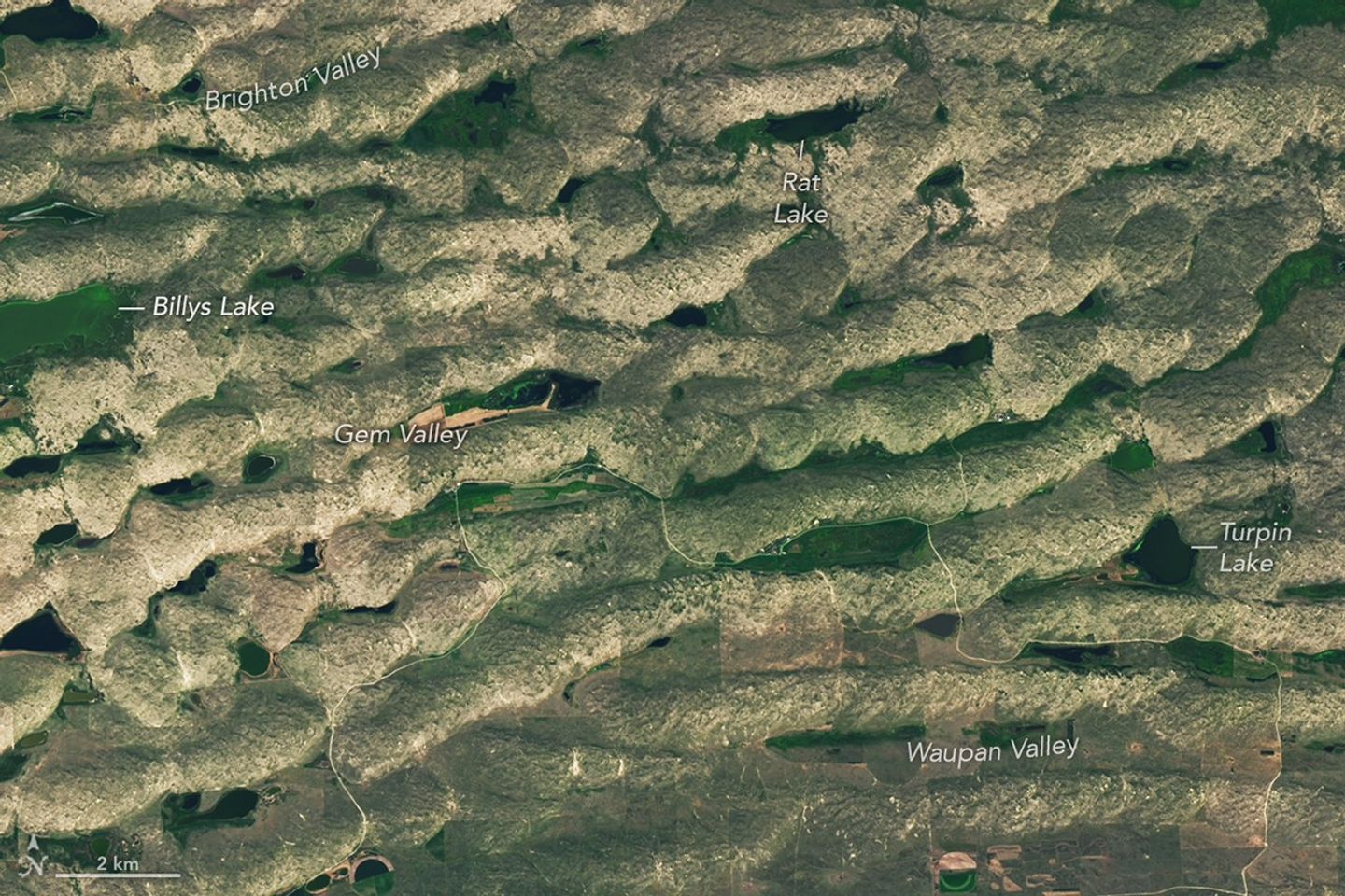
Some of the largest, grassland-covered dunes in the Nebraska Sandhills are found in the northwestern part of the region, shown in this image acquired on August 19, 2025, with the OLI (Operational Land Imager) on Landsat 8.
NASA Earth Observatory/Lauren Dauphin
Some of the largest dunes occur in and around the area shown in the detailed image above, near the northern edge of the Sandhills region. These transverse dunes stand as high as 400 feet (120 meters) and extend for several miles. Their northern slopes are gentler than their southern slopes, reflecting the dominant influence of northerly winds. In other areas, dunes are more symmetric, suggesting that winds blew with nearly equal strength from the north and south, alternating with the seasons.
The grasslands that now cover the hills constitute pastureland for grazing livestock. Ranching expanded significantly in the area after passage of the Kinkaid Act in 1904, which allotted 640-acre parcels of land to ranchers who would settle it. Today, far more cattle than humans occupy the region, and half of Nebraska’s nearly 23 million acres of rangeland and pastureland are in the Sandhills. Some ranchers graze their cattle in patterns meant to approximate the large bison herds that once roamed the land.
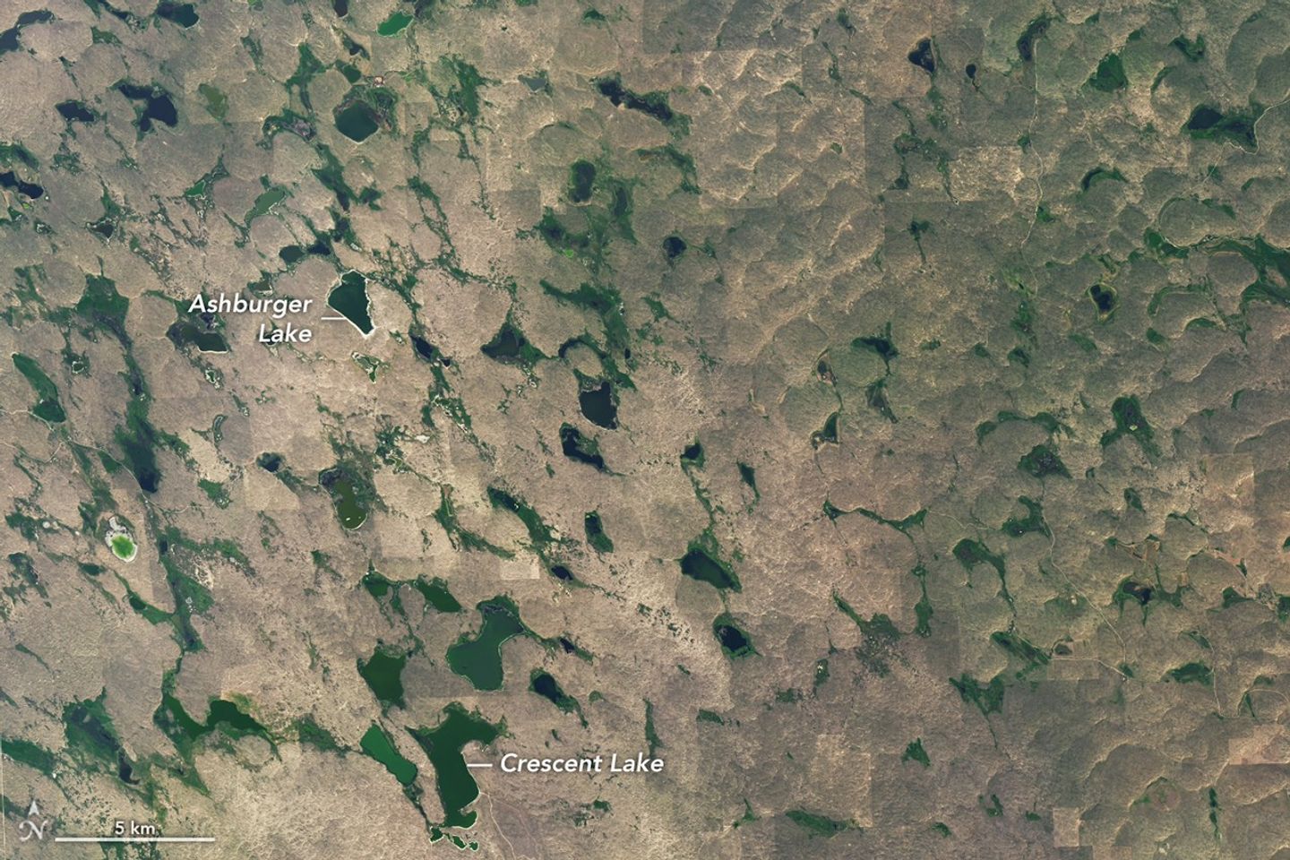
Lakes and wetlands fill the valleys between dunes in Crescent Lake National Wildlife Refuge, shown in this image acquired on August 19, 2025, with the OLI (Operational Land Imager) on Landsat 8.
NASA Earth Observatory/Lauren Dauphin
Though much of the land in the Sandhills is privately owned, some is set aside in protected public lands. One of these areas, Crescent Lake National Wildlife Refuge on the southwestern edge of the Sandhills region, is shown above. Wetlands, including shallow lakes, marshes, and wet meadows, fill some of the valleys between the dunes. The land here is sponge-like, with precipitation seeping down through the soil and recharging groundwater instead of flowing off through stream channels.
Located along the Central Flyway, the refuge is a haven for migratory birds, and dozens of species of waterfowl, marsh birds, and shorebirds utilize the area. Among other wildlife, several types of turtles thrive in the ponds and prairies. Wetlands across the Sandhills support rare species such as the whooping crane, western prairie fringed orchid, and Topeka shiner.
NASA Earth Observatory images by Lauren Dauphin, using Landsat data from the U.S. Geological Survey. Story by Lindsey Doermann.

 Login