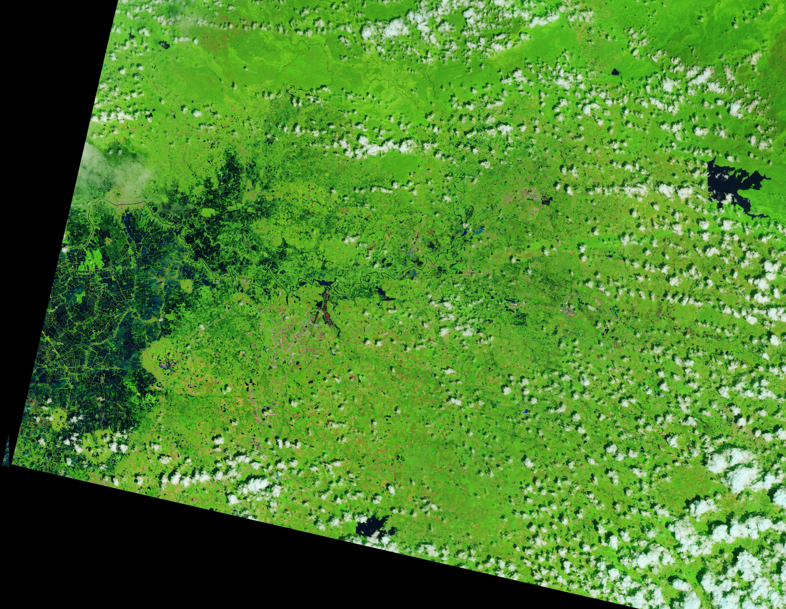
A narrow river (dark blue) meanders across vegetated land (bright green) in a false-color satellite image. Small geometric ponds or waterlogged fields appear on the left side of the scene.
NASA Earth Observatory / Lauren Dauphin
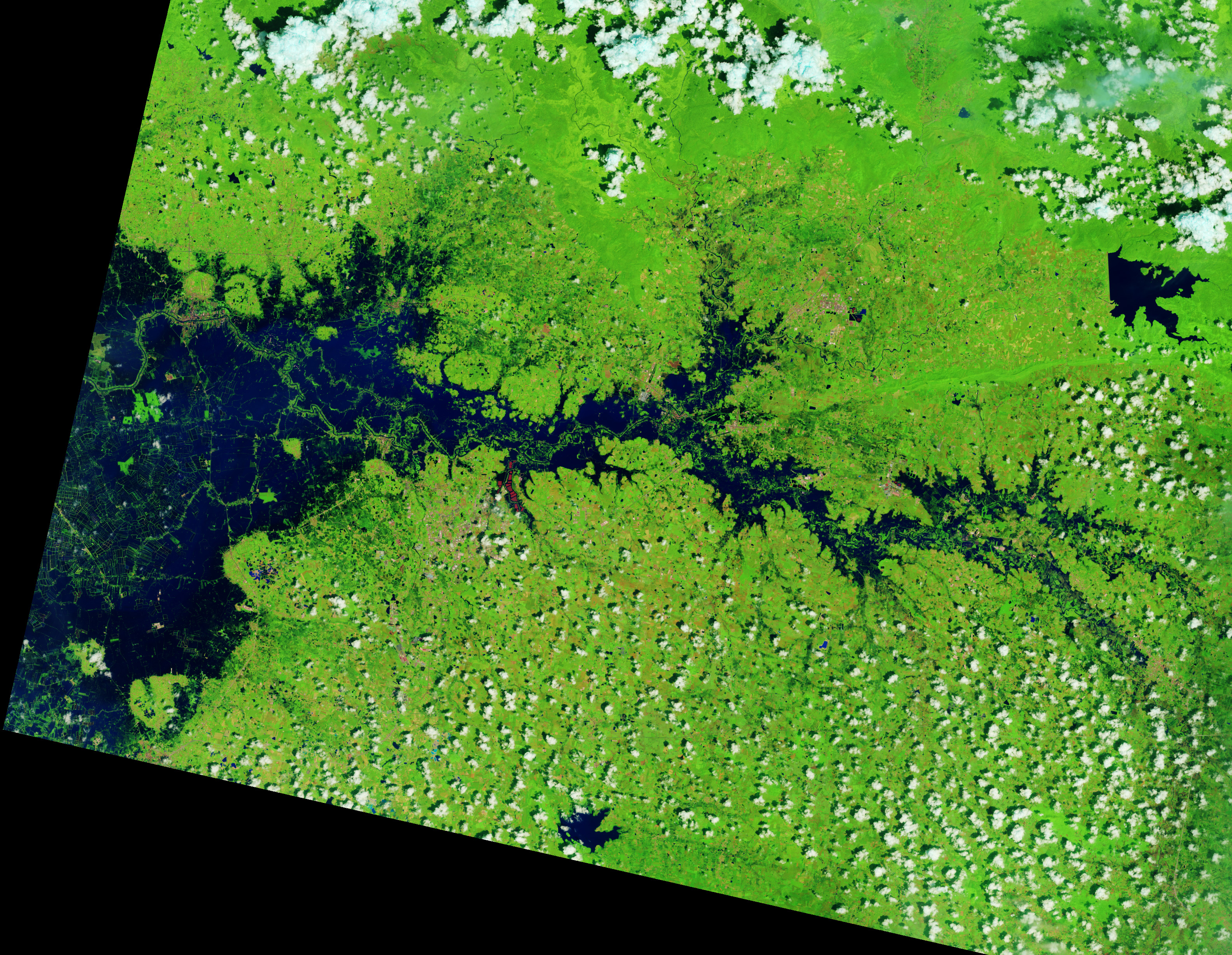
In a false-color satellite image of the same area, floodwaters (dark blue) flank a meandering river and cover a large swath of agricultural or aquacultural land primarily on the left side of the scene.
NASA Earth Observatory / Lauren Dauphin
October 7, 2025
October 2, 2026
September falls in the heart of the monsoon season in Thailand, where cities and towns are accustomed to the afternoon rains and thunderstorms that frequently roll through. But throughout late September and early October 2026, persistent heavy rains punctuated by intense downpours left low-lying areas across the country in Southeast Asia under sustained flooding.
Prachin Buri province was among the areas where flooding was widespread. The right image above shows land along the Bang Pakong River and nearby agricultural areas and aquaculture facilities inundated on October 2, 2026. The left image shows the same area at the same time of year in 2025. Acquired with NASA-USGS Landsat satellites, the images are false-color to better distinguish water from vegetation, developed land, and other surfaces. The bright red shapes are floating solar arrays.
Some of the flooding likely stemmed from a low-pressure system that stalled over the area for several days in late September. Stoked by moisture and energy from the warm Gulf of Thailand nearby, the system delivered especially intense rains to the region. About 100 kilometers (60 miles) to the west, Bangkok received nearly 300 millimeters (11.8 inches) of rain over a 48-hour period, according to news reports, close to the average monthly rainfall total for September of 344 millimeters (13.5 inches).
Since mid-September, flooding has occurred in 50 provinces across the country, affecting over 4 million people and causing dozens of deaths, according to the International Federation of Red Cross and Red Crescent Societies. Government agencies estimate about 270,000 hectares (670,000 acres) of farmland, including rice fields and fruit orchards, have been damaged.
NASA Earth Observatory images by Lauren Dauphin, using Landsat data from the U.S. Geological Survey. Story by Lindsey Doermann.
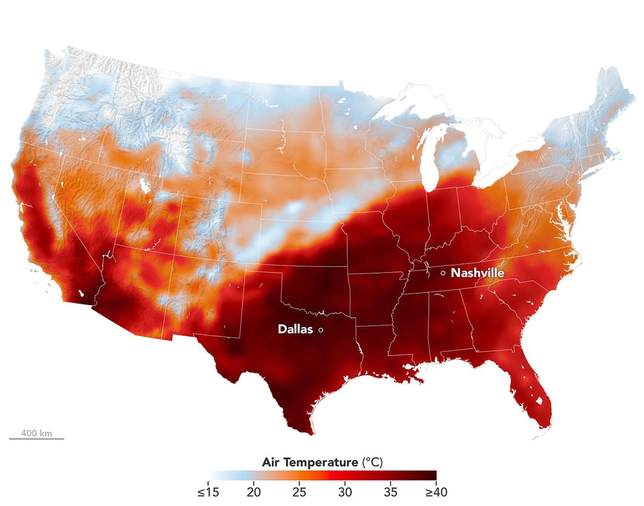
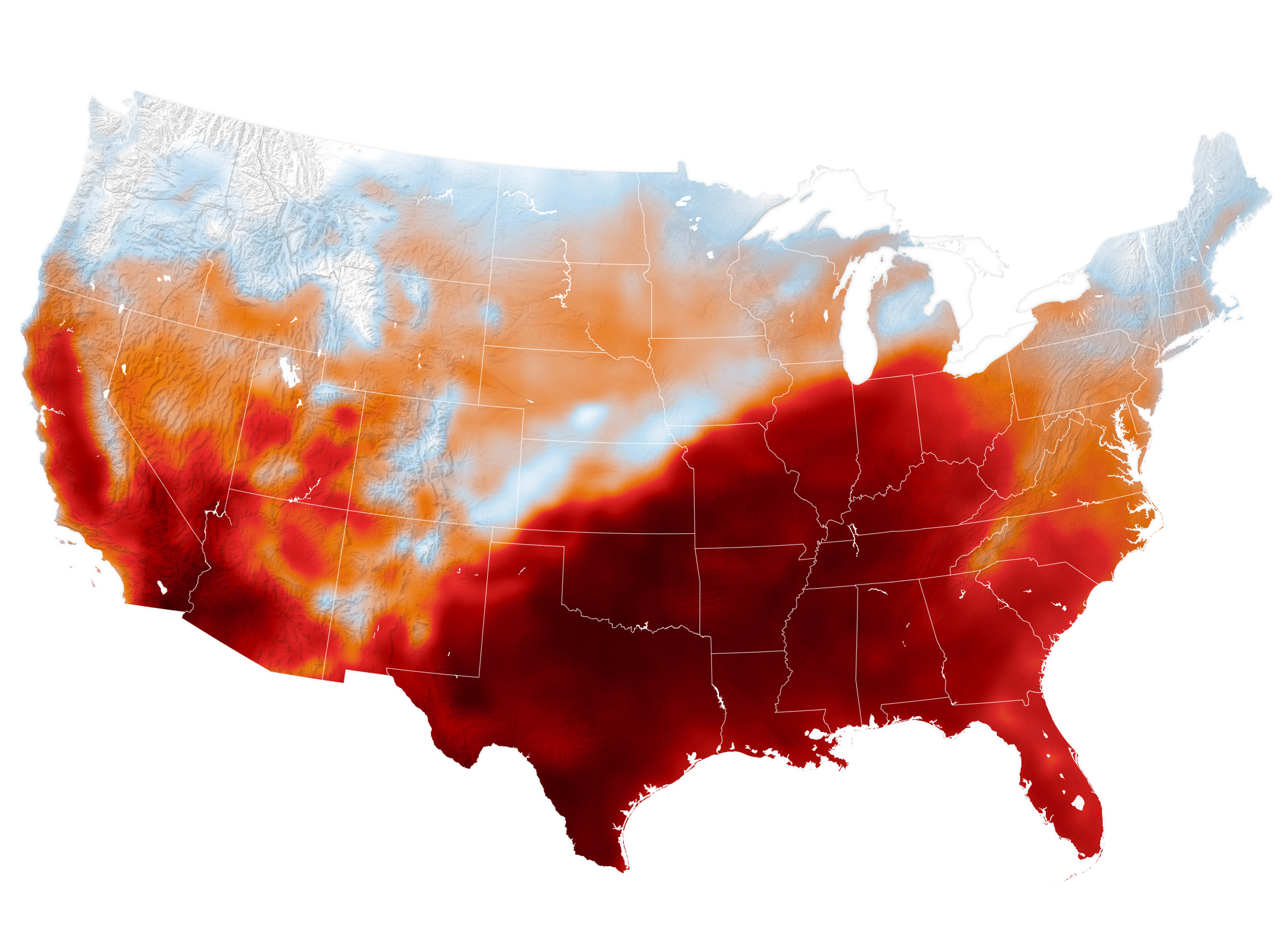
An area of high pressure over the south-central U.S. produced unseasonable and, in some places, record-breaking warmth on September 15, 2026, as shown in this map of modeled air temperatures from GEOS (Goddard Earth Observing System).
NASA Earth Observatory/Michala Garrison
While the calendar indicated that astronomical summer was winding down, a swath of the south-central United States was sweltering under a heat dome in mid-September 2026.
This map shows air temperatures in the contiguous U.S. on September 15, 2026, at 4 p.m. Central Time (21:00 Universal Time), modeled at 2 meters (6.5 feet) above the ground. It was produced by combining satellite observations with temperatures predicted by a version of the GEOS (Goddard Earth Observing System) model, which uses mathematical equations to represent physical processes in the atmosphere. The darkest reds indicate areas where temperatures approached or exceeded 40 degrees Celsius (104 degrees Fahrenheit).
More than 41 million people in the U.S.—about 12 percent of the population—were under a National Weather Service extreme heat advisory, extreme heat watch, or extreme heat warning on September 15. The high temperatures spanned large portions of several states, such as Texas, Oklahoma, Arkansas, Missouri, and Tennessee. Meteorologists warned that high humidity, limited cloud cover, and light winds could make temperatures feel higher than thermometer readings and increase the risk of heat-related illnesses.
Several locations set new daily high temperature records on September 15. These included Dallas, Texas, at 101ºF (38ºC), Memphis, Tennessee, at 99ºF (37ºC), and Nashville, Tennessee, at 100ºF (38ºC). The cities were all at least 12ºF warmer than normal that day, with Nashville breaking its daily-high record from 1927. The day before, Nashville also set a record-high minimum temperature of 75ºF (24ºC).
A weather phenomenon meteorologists call a heat dome was responsible for driving temperatures up across the region. A heat dome develops when an area of high pressure in the upper atmosphere pushes hot air toward the surface and traps it there. Heat domes put the brakes on convection and suppress clouds and precipitation. This allows sunlight to reach Earth’s surface relatively unhindered and further elevate air temperatures.
The stretch of unseasonable temperatures follows the warmest June through August in the contiguous United States in a 132-year record, according to NOAA. The three-month period in 2026 was 0.4ºF warmer than the previous records, set in 1936 and 2021.
One of the inspirations for Jimi Hendrix’s iconic 1967 hit “Purple Haze” is said to be the sci-fi novelNight of Light, about a distant planet in a binary star system. Every seven years, the story goes, the stars bathe the planet in a bizarre purple radiance with the power to rearrange physical reality in profound and unexpected ways. The atmosphere’s purple glow, for instance, turned some people into trees and brought statues to life.
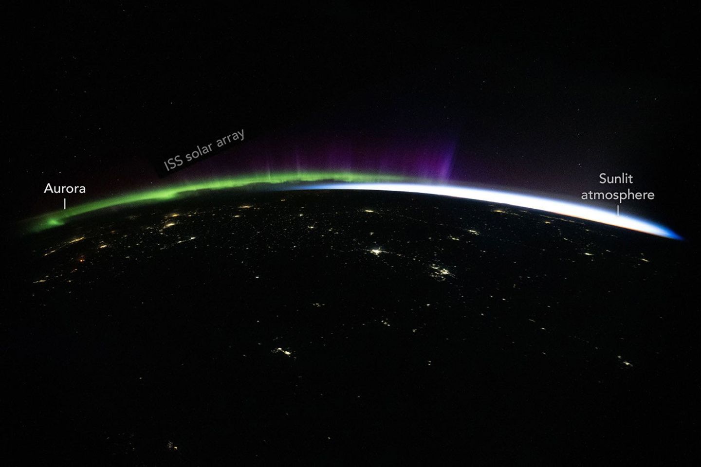
It’s perhaps fitting, then, for an astronaut on the International Space Station to invoke the iconic song after witnessing the aurora illuminate Earth’s atmosphere with ethereal greens, reds, and purples. Hendrix would have “rejoiced” at the “brilliant purple,” NASA astronaut Jessica Meir posted on September 8. It “makes me want to kiss the sky,” she added in a nod to the lyrics of the Hendrix song.
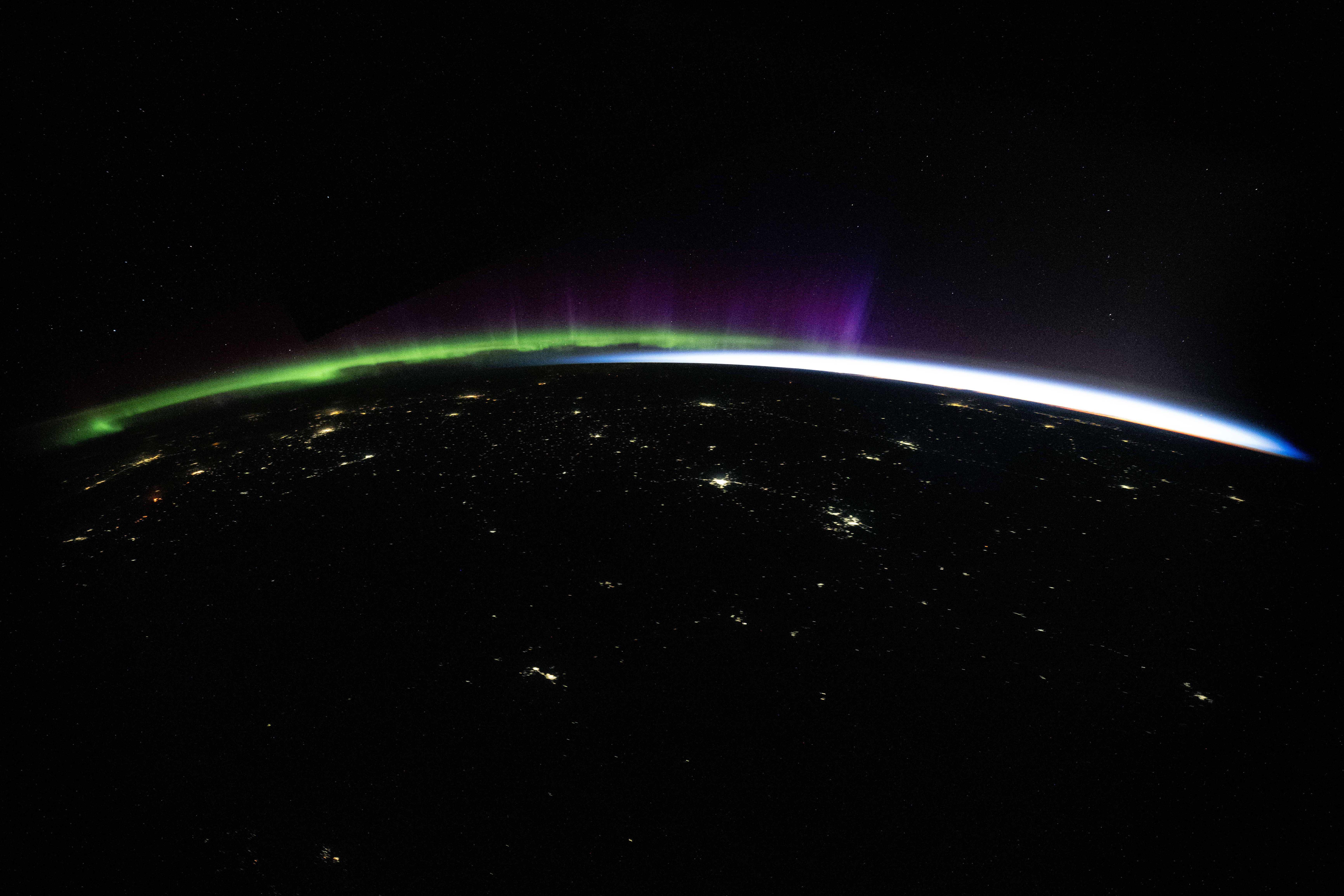
The photograph above is one of many that the astronauts took on September 7, 2026, as they orbited an atmosphere quivering with color. The station was at an altitude of 255 miles (411 kilometers) and above Kyrgyzstan when the photo was taken. Stacking several of the photos also yielded a long-exposure series in which the aurora’s green glow mingles with star trails, moonlight, passing satellites, and city lights in a dazzling jumble of illumination.
Aurora is the Latin word for “dawn” and also the name of the Roman goddess of the dawn. Its use in reference to the atmospheric phenomenon likely comes from Europeans living far from the Arctic Circle, who would have experienced the aurora as a faint red glow to the north, resembling the reddish glow in the east at dawn.
The colorful phenomenon typically starts when the Sun sends charged particles toward Earth through solar flares, coronal mass ejections (CMEs), or an active solar wind. These particles interact with the magnetosphere—the invisible, comet-shaped bubble of magnetic field lines surrounding the planet—compressing and changing the configuration of the magnetic field. In the process, some particles within the field are drawn into Earth’s upper atmosphere, where they excite nitrogen and oxygen atoms and molecules, causing them to release photons.
The colors of auroras are influenced by the type of gas involved and the altitude at which they occur in the atmosphere. Oxygen excited to different energy levels can produce green and red. Green occurs roughly between 60 and 120 miles (100 and 200 kilometers) altitude, and red occurs above 120 miles (200 kilometers). Excited nitrogen gas, from about 60 to 120 miles (100 to 200 kilometers), glows blue or pink depending on the type and energy of the particles it interacts with. Sometimes, the light emitted by gases can appear to mix, making the auroras seem purple, pink, or even white.
While auroras can occur any time of the year, astronauts are especially likely to enjoy the light shows in the spring and fall, around the equinoxes. That’s because the geometry of Earth’s magnetic field relative to the solar wind makes it especially favorable for transferring solar-wind energy into the magnetosphere, a phenomenon known as the Russell-McPherron effect.
This isn’t the only example of Jimi Hendrix’s music making an impression beyond Earth. A selection of Hendrix’s music touched down on the Moon in 2024 with the Odysseus lander. Another Hendrix song, “Voodoo Chile,” made the list of wake-up songs for STS-110, according to a report from NASA’s History Division.
Astronaut photographISS075-E-88592 was acquired on September 7, 2026, with a Nikon Z9 digital camera using a focal length of 15 millimeters. It is provided by the ISS Crew Earth Observations Facility and the Earth Science and Remote Sensing Unit at NASA Johnson Space Center. The image was taken by a member of the Expedition 75 crew. The image has been cropped and enhanced to improve contrast, and lens artifacts have been removed. The International Space Station Program supports the laboratory as part of the ISS National Lab to help astronauts take pictures of Earth that will be of the greatest value to scientists and the public, and to make those images freely available on the internet. Additional images taken by astronauts and cosmonauts can be viewed at the NASA/JSC Gateway to Astronaut Photography of Earth. Story by Adam Voiland.
In August 2026, a series of powerful winter storms transformed parts of northern Chile’s Atacama Desert, covering the famously dry landscape in an unusual layer of snow. Snow is not unheard of in the Atacama. Significant falls occurred in 2025 and, before that, in 2011. But one of the August 2026 storms stood out because [...]
The curving, parallel mountain ridges of the Sierra Madre Oriental are an eye-catching feature of northeastern Mexico’s landscape. The spot where these folds nestle up against Mexico’s second-largest metropolitan area captured the attention of an astronaut aboard the International Space Station, who took this photo on August 26, 2026.
Monterrey, the capital of the state of Nuevo León, is an industrial hub supporting heavy industries such as ironworks and steelworks, as well as manufacturing facilities for goods ranging from textiles to processed foods to glass and plastics. The metropolitan area is home to 5.3 million people, according to the 2020 census. And while the city has seen overall population growth since 1990, the number of people living within 5 kilometers (3 miles) of the city center has declined, researchers have found—a trajectory shared with many of Mexico’s metropolitan areas.
In Monterrey’s case, urban expansion runs up against some unforgiving terrain. Along the city’s southern edge, layers of limestone, deposited in the late Mesozoic era and then folded between about 80 and 50 million years ago, form the Sierra Madre Oriental. Over millions of years, weaker rock layers have eroded away, leaving behind the distinct ridgelines that bound Monterrey today.
The Río Santa Catarina carves through the mountains and onto the semiarid floodplain where the city lies. Because of the dry environment, the river carries little to no water for much of the time. But its channel is crucial for collecting runoff from summer rains and serves as an important natural area for plant and animal life within the city.
The river runs through Monterrey’s urban core and between several island-like protrusions of folded rock. One of these is the Sierra Las Mitras, a state nature reserve established in 2000. The mountain ridge rises approximately 1,500 meters (4,900 feet) over the city and provides a haven for wildlife. As conditions become cooler and wetter with higher elevations, vegetation turns from cacti and thorny shrubs on lower rocky slopes to oak and pine forests higher on the ridge. Cerro de la Silla (Mount Silla or Saddle Hill) is another prominent feature of the landscape, contrasting with the built environment.
Near the city’s border with the Sierra Madre Oriental sits Universidad de Monterrey, a host venue for the NASA Space Apps Challenge. This annual hackathon will take place in November 2026 in person and virtually at sites around the world. Participating teams use NASA and partner agency data to tackle challenges in fields such as software development, astrophysics, space exploration, and agriculture.
Astronaut photograph ISS075-E-70481 was acquired on August 26, 2026, with a Nikon Z9 digital camera using a focal length of 400 millimeters. It is provided by the ISS Crew Earth Observations Facility and the Earth Science and Remote Sensing Unit at NASA Johnson Space Center. The image was taken by a member of the Expedition 75 crew. The image has been cropped and enhanced to improve contrast, and lens artifacts have been removed. The International Space Station Program supports the laboratory as part of the ISS National Lab to help astronauts take pictures of Earth that will be of the greatest value to scientists and the public, and to make those images freely available on the internet. Additional images taken by astronauts and cosmonauts can be viewed at the NASA/JSC Gateway to Astronaut Photography of Earth. Story by Lindsey Doermann.
Puerto Rico went from no drought to widespread extreme drought in just months as rainfall collapsed and water shortages spread. Puerto Rico usually enters its wet season in May. In 2026, however, the expected rains largely failed to arrive through late August, leaving much of the U.S. territory in drought. The prolonged dry spell has [...]
A giant 29-square-mile iceberg broke from Greenland’s Petermann Glacier and survived a collision with Joe Island that might have shattered a more fragile berg. Summer is the busiest time of year for iceberg activity in Greenland’s glacier-fed fjords, and 2026 brought another dramatic example. In August, a huge iceberg separated from Petermann Glacier on Greenland’s [...]
New Mexico’s largest reservoir plunged to just 1.4 percent capacity in July 2026, revealing the dramatic impact of prolonged drought and record early snowmelt. NASA is using satellite data to help water managers understand the shrinking supply and prepare for future shortages. When astronaut John Glenn remarked on the landscape below him while orbiting Earth [...]
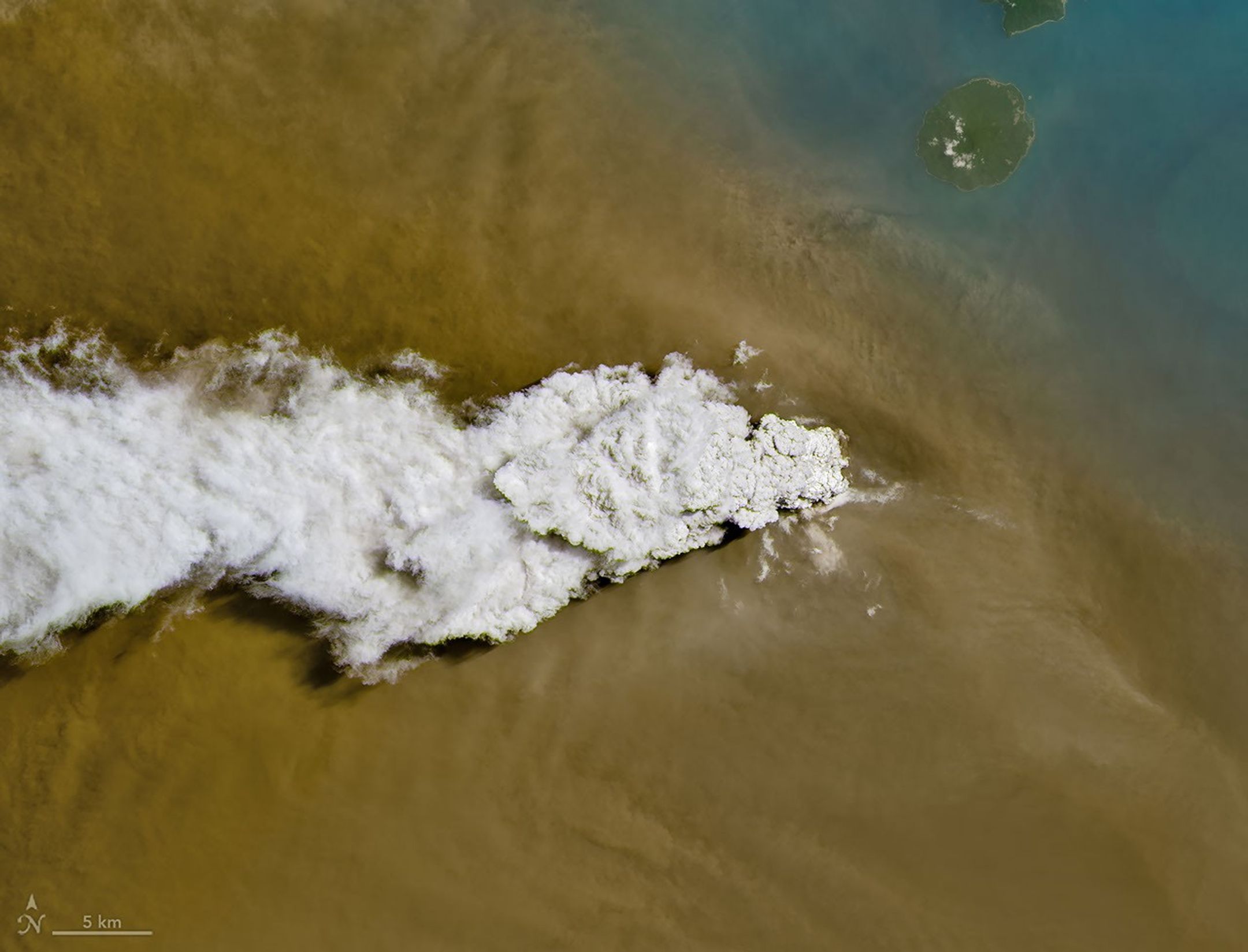
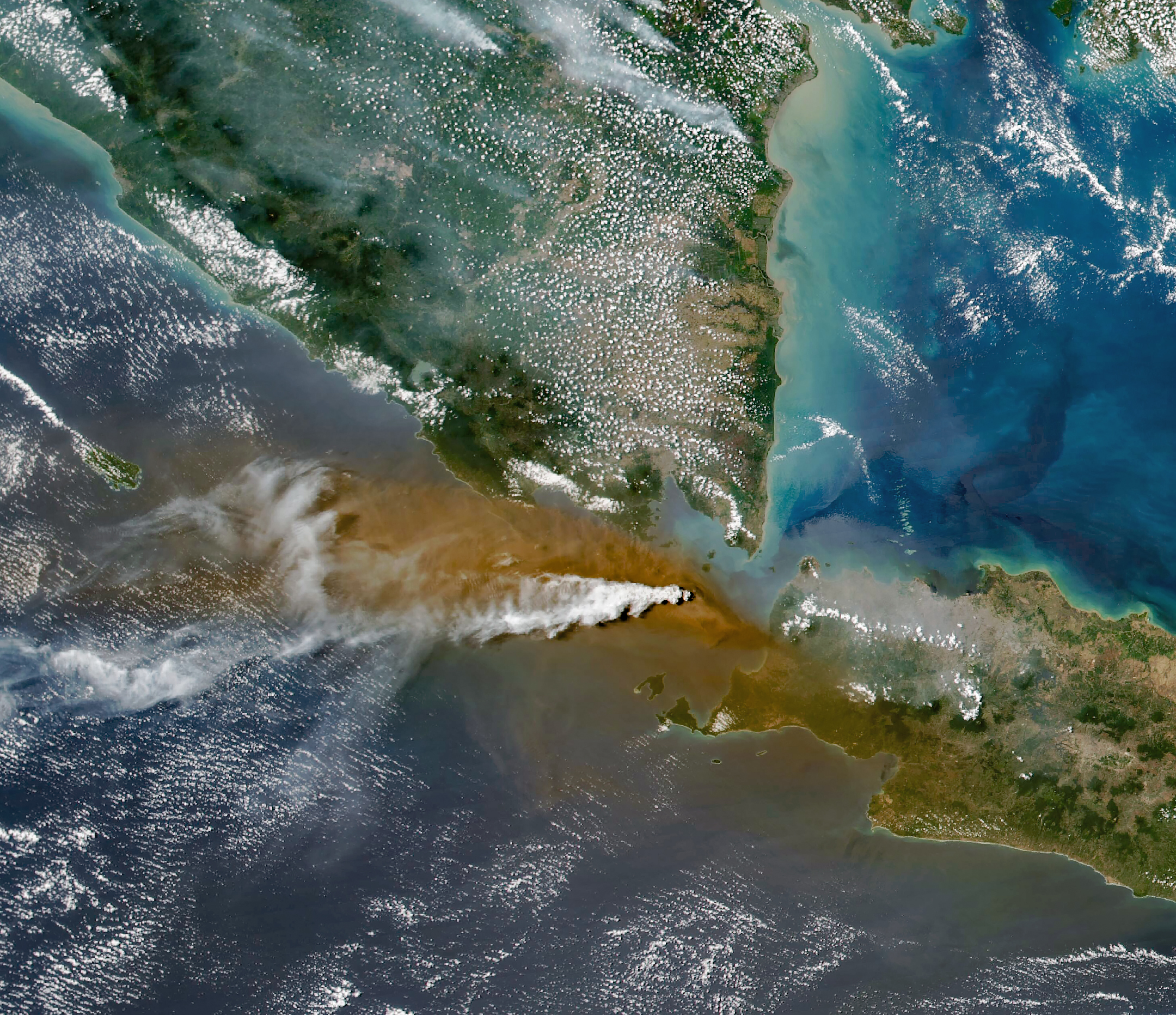
Anak Krakatau erupts ash and volcanic gases in this image acquired with the OLI (Operational Land Imager) on Landsat 8 on September 5, 2026.
NASA Earth Observatory/Michala Garrison
Eruptions are a regular occurrence at Anak Krakatau, a small volcano between the Indonesian islands of Java and Sumatra. Much of its activity remains relatively mild, but it occasionally puts on more impressive and hazardous shows of force. In early September 2026, a booming eruption lasting more than 24 hours sent gas and ash high into the atmosphere, disrupting thousands of flights and degrading air quality in parts of the country, including the capital city of Jakarta.
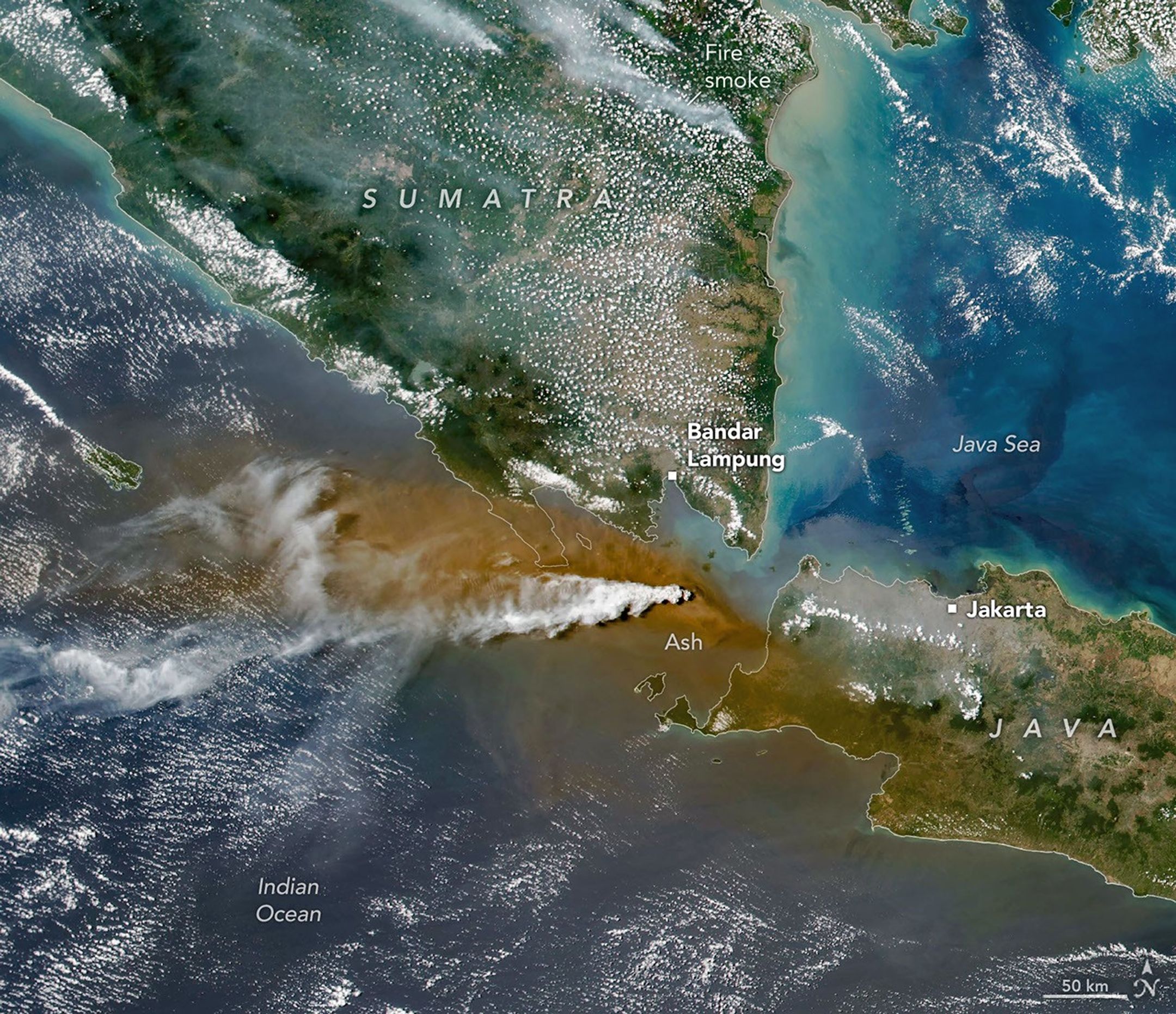
Satellites passing over the area during the eruption on September 5 captured images of the explosive activity. In the scene above, acquired with the OLI (Operational Land Imager) on the NASA-USGS Landsat 8 satellite, a white plume of volcanic gas billows over a brown ash cloud. Below, a wider view captured by the VIIRS (Visible Infrared Imaging Radiometer Suite) on the Suomi NPP satellite shows the volcanic material dispersing over a large area.
Indonesia’s meteorological agency reported that ash had reached altitudes up to 6,000 meters (20,000 feet) to the east of the volcano and 15,000 meters (50,000 feet) to the west by September 6. The presence of ash in the atmosphere prompted the temporary closure of eight airports on Java and Sumatra, disrupting nearly 3,000 flights in and out of the area, according to news reports.
Plumes of ash and volcanic gases from Anak Krakatau drift over Indonesia and the Indian Ocean in this image captured by the VIIRS (Visible Infrared Imaging Radiometer Suite) on the Suomi NPP satellite on September 5, 2026.
NASA Earth Observatory/Michala Garrison
Ashfall affected populated areas, particularly to the east of Anak Krakatau in Jakarta and other parts of West Java, the Indonesian Humanitarian Coordination Platform (IHCP) reported. Volcanic ash poses health risks to people and can irritate the respiratory tract, eyes, and skin. However, this air quality hazard differs from the smoke produced by peatland fires elsewhere in the country in terms of particle characteristics, dispersal patterns, and protection measures, the IHCP noted.
On September 6, the continuous explosive eruption from Anak Krakatau subsided, though the volcano kept rumbling. It returned to a more typical pattern of Strombolian eruptions, characterized by intermittent spurts of ash and volcanic material. Airports had resumed operation by September 8, but the volcano remained at the second-highest alert level on the country’s scale, as it has been since early July.
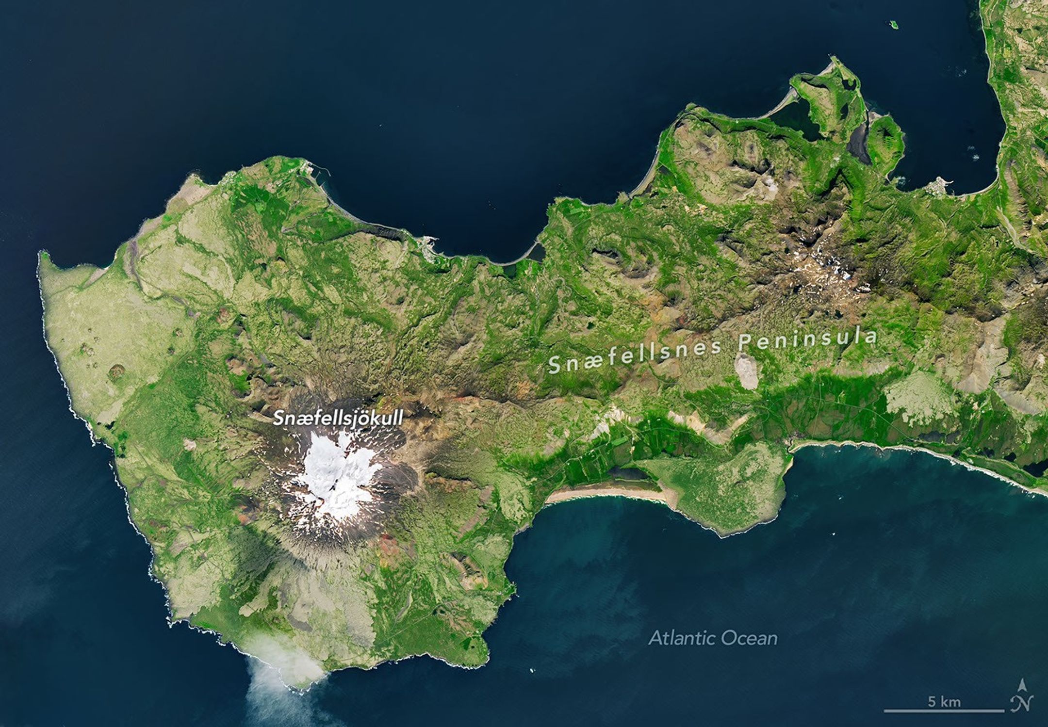
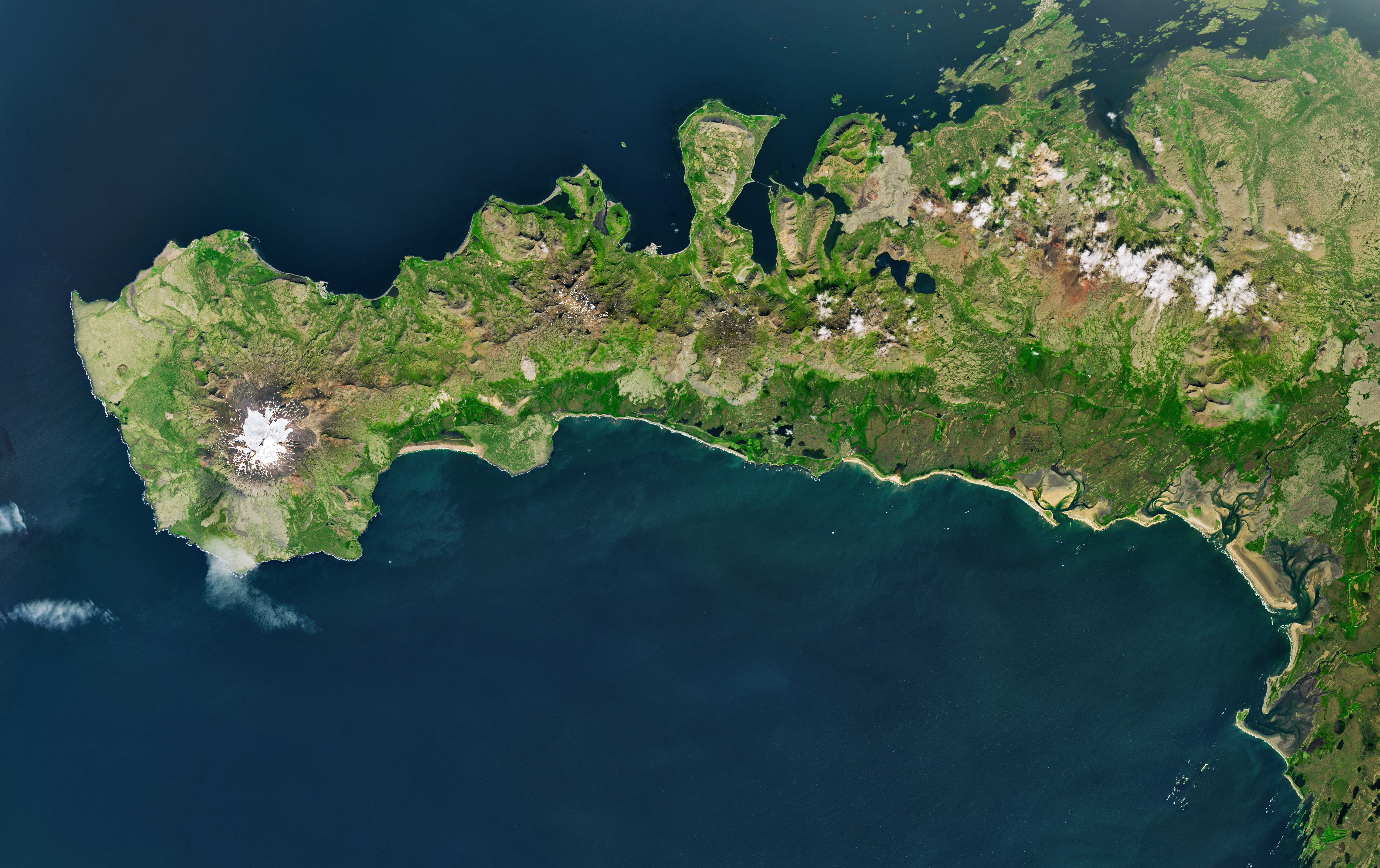
The glacier-capped Snæfellsjökull volcano is the defining feature of Iceland’s Snæfellsnes peninsula, shown in this image acquired with the OLI (Operational Land Imager) on Landsat 9 on July 25, 2026.
NASA Earth Observatory/Michala Garrison
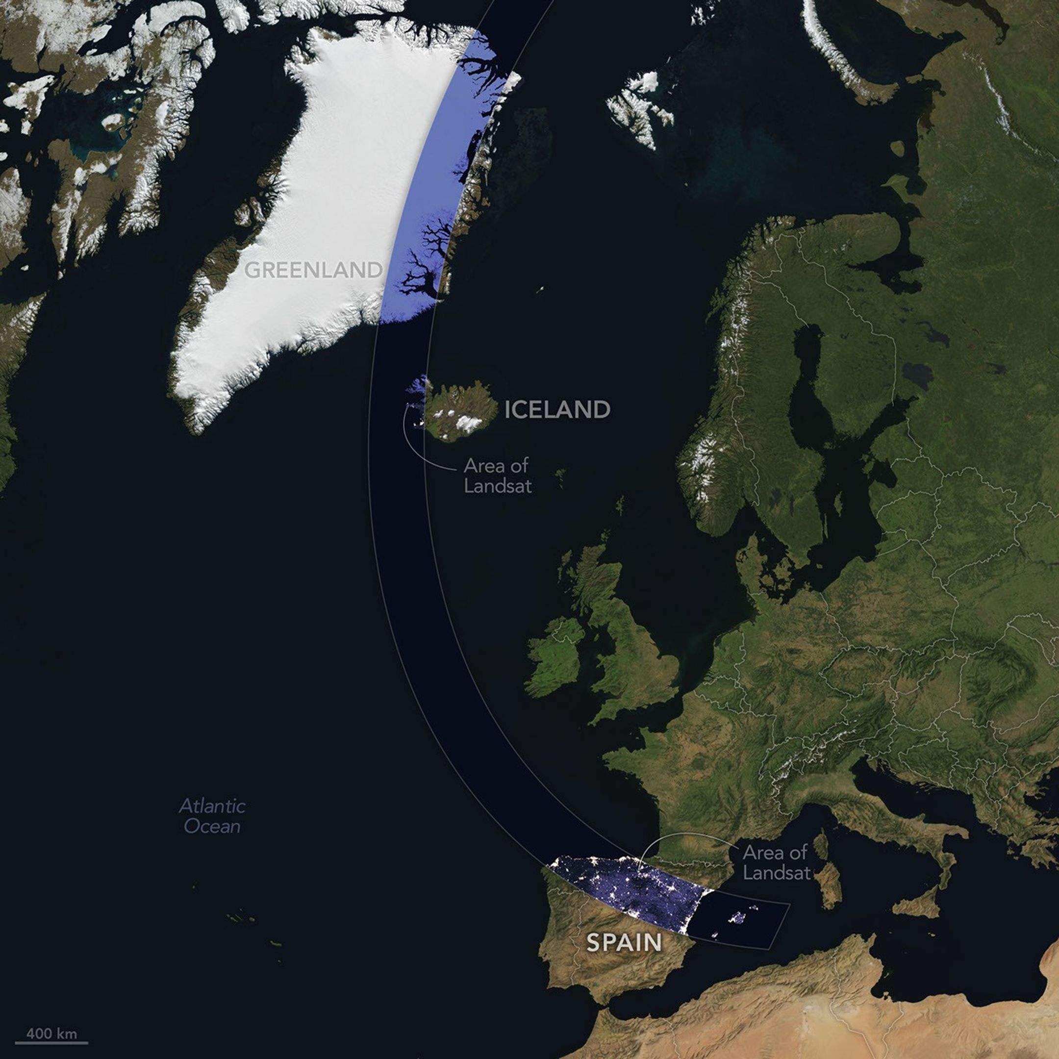
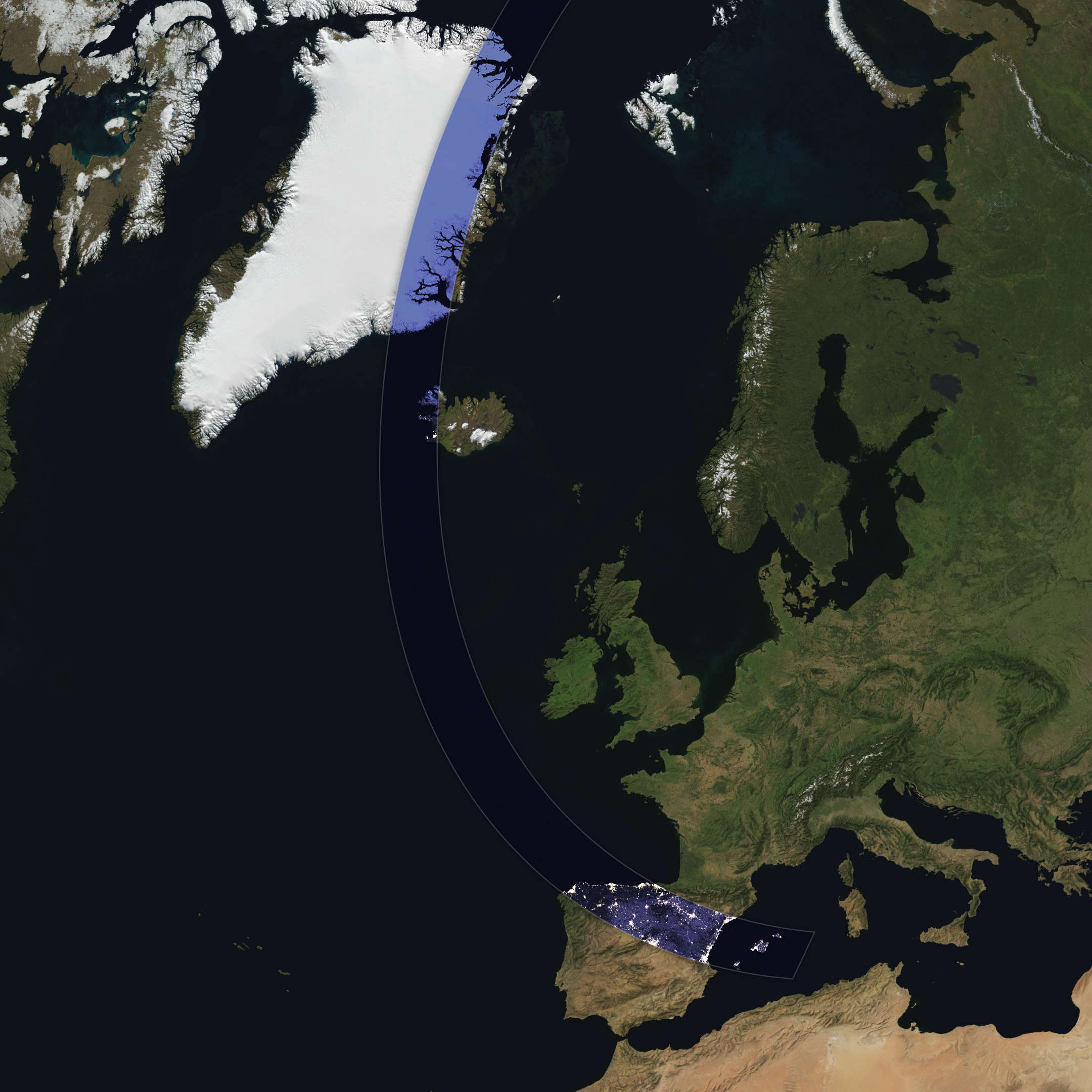
The Sun, Moon, and Earth align on August 12, 2026, to produce a total solar eclipse. When this celestial event last occurred, on April 8, 2024, the path of totality stretched across North America, giving millions the chance to glimpse the Sun’s corona. In 2026, the viewing locales are more limited; only a handful of land areas in the Northern Hemisphere, including parts of Iceland and Spain, fall within the path of totality.
On August 12, the Moon’s shadow will first cross over the Arctic Circle from northern Russia and then track along the eastern side of Greenland. At about 5:45 p.m. local time in Iceland (17:45 Universal Time), the country’s western fringes—including the Snæfellsnes peninsula, shown in the Landsat image above—will begin to experience totality. The greatest eclipse will occur near this sparsely populated peninsula when the Moon appears the largest and covers more of the Sun.
The path of totality of the solar eclipse on August 12, 2026, spans Greenland, Iceland, and Spain. The base imagery for the map comes from Blue Marble: Next Generation, with data from Black Marble shown in the path of totality. Blue Marble is built from scenes captured by MODIS (Moderate Resolution Imaging Spectroradiometer), while Black Marble is based on observations by the VIIRS (Visible Infrared Imaging Radiometer Suite) day-night band.
NASA Earth Observatory/Michala Garrison
The Snæfellsjökull volcano on the western end of the peninsula is covered in ice and last erupted about 1,800 years ago. It is the highlight of a national park of the same name, where people are expected to visit to view the eclipse. The stratovolcano even has a literary claim to fame: in Jules Verne’s A Journey to the Center of the Earth, characters venture underground through its crater, later emerging in an eruption of Stromboli, in Italy. In 2025, a broader area of the peninsula was designated a UNESCO biosphere reserve, containing over 70 percent of Iceland’s flora and an agglomeration of volcanic landscapes, wetlands, and grasslands.
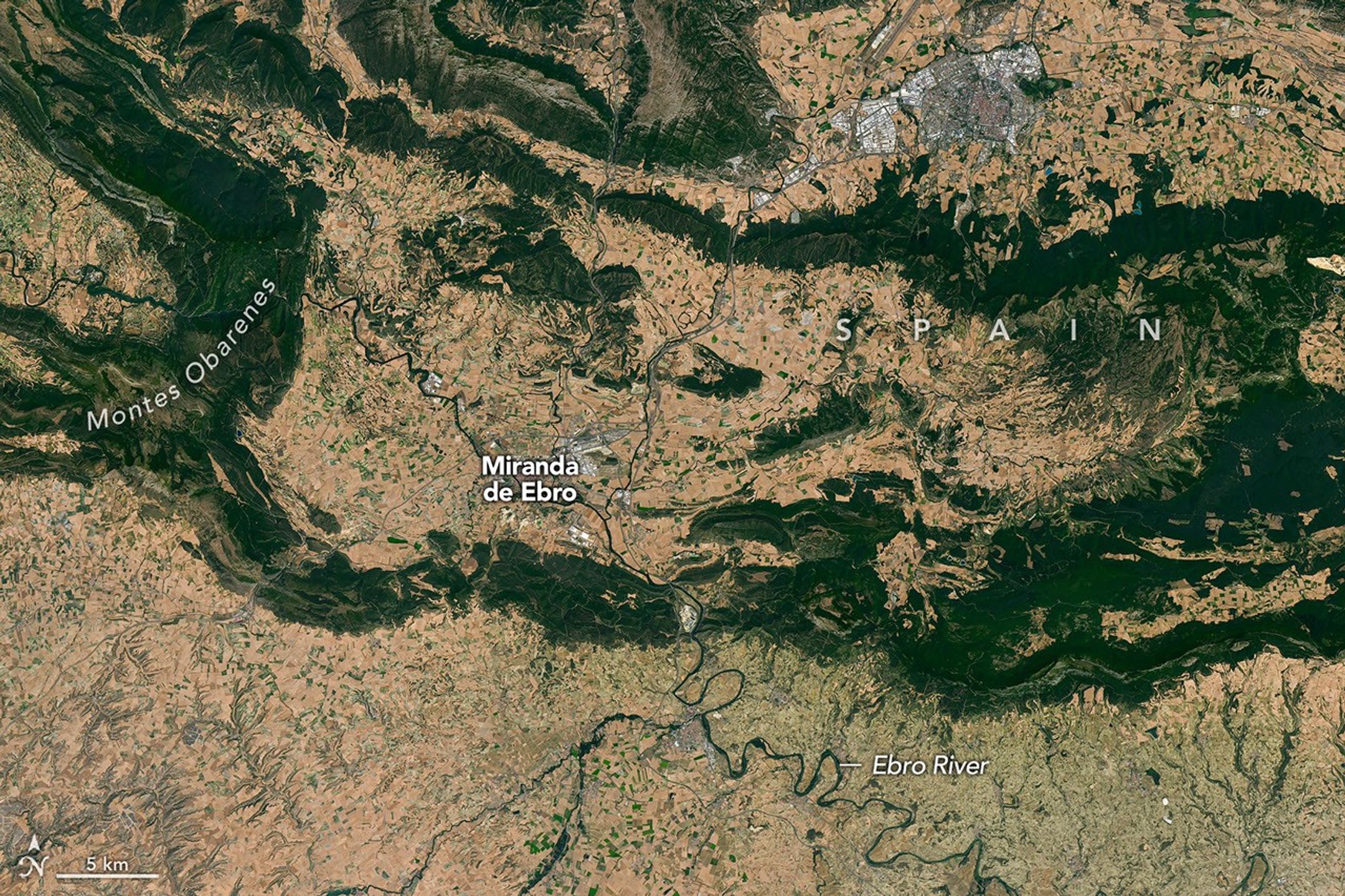
From Iceland, the eclipse shadow, or umbra, progresses across the North Atlantic and reaches northern Spain shortly before sunset. It runs east-southeast across the country, much like the Ebro River (Río Ebro), seen in the Landsat image below.
The Ebro River, meandering across northern Spain in this image acquired with the OLI (Operational Land Imager) on Landsat 8 on July 21, 2026, is in the path of totality of the August 2026 solar eclipse.
NASA Earth Observatory/Michala Garrison
The upper Ebro emerges from rugged terrain in Parque Natural de Montes Obarenes-San Zadornil, where it carves canyons and gorges through the eastern foothills of the Cantabrian Mountains. It then meanders through La Rioja, a region known for its vineyards. About 400 kilometers (250 miles) away, the river reaches a delta on the Mediterranean coast between Barcelona and Valencia.
Based on satellite measurements of cloud cover in August over several decades, viewers in Spain have a higher likelihood than those in Iceland of getting a clear look at the eclipse. And despite limited viewing opportunities in the path of totality, the rest of Europe, parts of Africa, Canada, and the northern and northeastern U.S. will experience a partial eclipse.
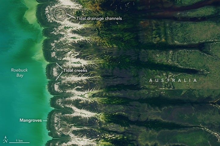
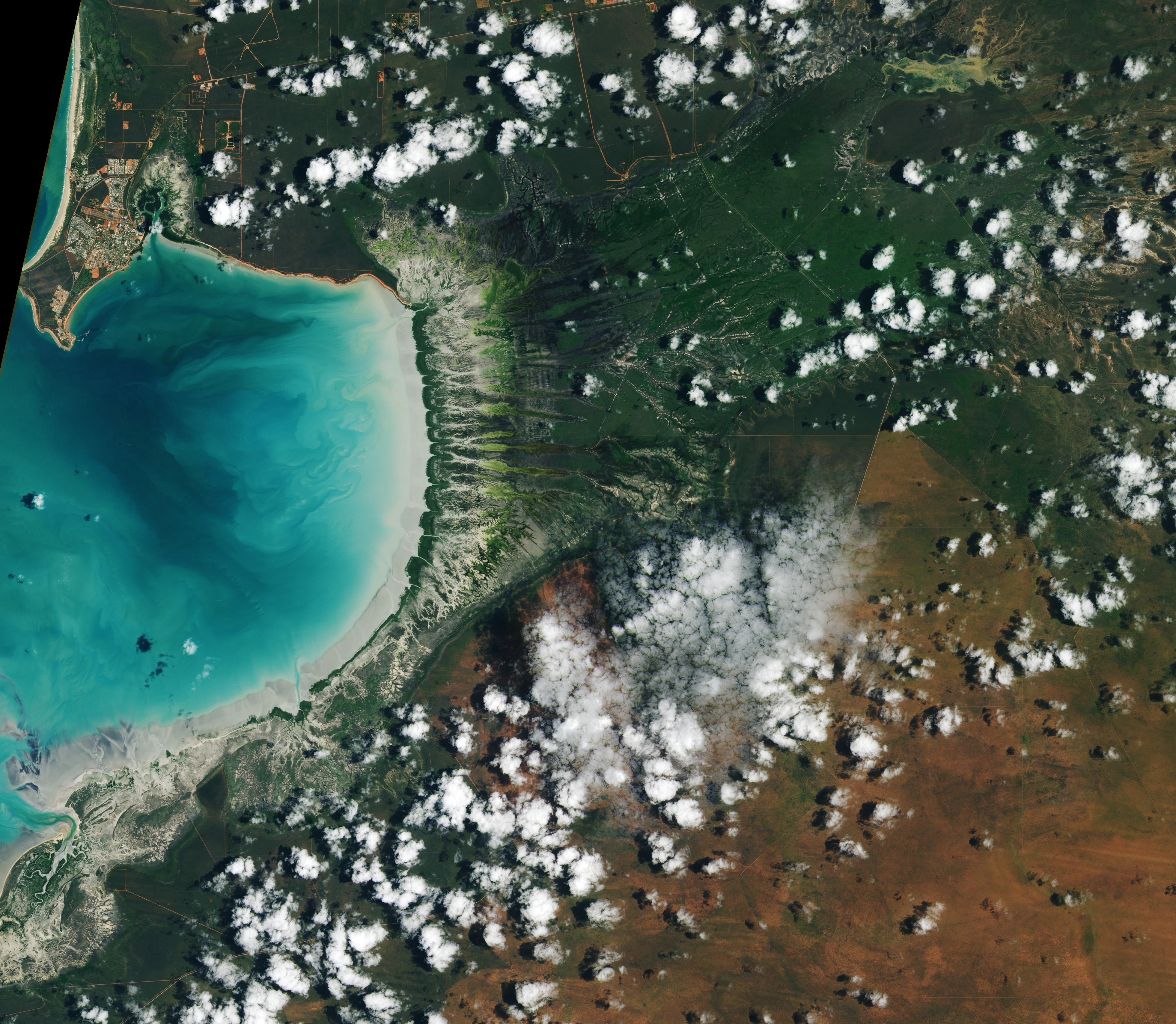
Water covers intertidal mudflats around Roebuck Bay in Western Australia, as seen in this image captured by the OLI (Operational Land Imager) on Landsat 8 on March 18, 2026.
NASA Earth Observatory / Lauren Dauphin
Editor’s Note: Today’s story is the answer to the August Puzzler.
Tides are among the clearest signs of the Moon’s pull on Earth. Just 239,000 miles (385,000 kilometers) away, the Moon’s gravity pulls on Earth’s oceans and solid crust, subtly distorting them into a more oblong shape with bulges roughly extending toward and away from the Moon.
High tides happen throughout Earth’s oceans, but in some places they leave an unusually strong fingerprint on the landscape. Among those places is Roebuck Bay, a crescent-shaped feature in the Kimberley region of Western Australia.
Roebuck Bay’s tidal range can reach a remarkable 9 meters (30 feet). Rising and falling tides repeatedly inundate and expose expansive mudflats, flood broad mangrove forests and salt marshes, and feed branching networks of tidal drainage channels. Many parts of Australia have tidal ranges of 2 meters or less. But the large range at Roebuck Bay is mostly a consequence of northwestern Australia’s unusually wide, shallow continental shelf, which helps amplify tides as they approach the coast.
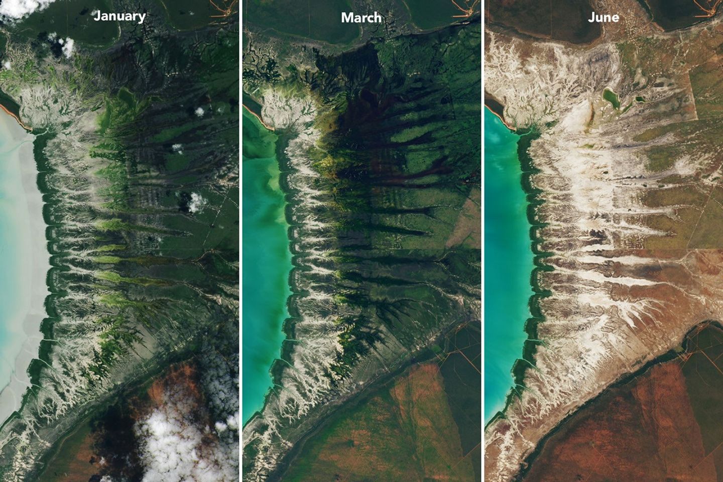
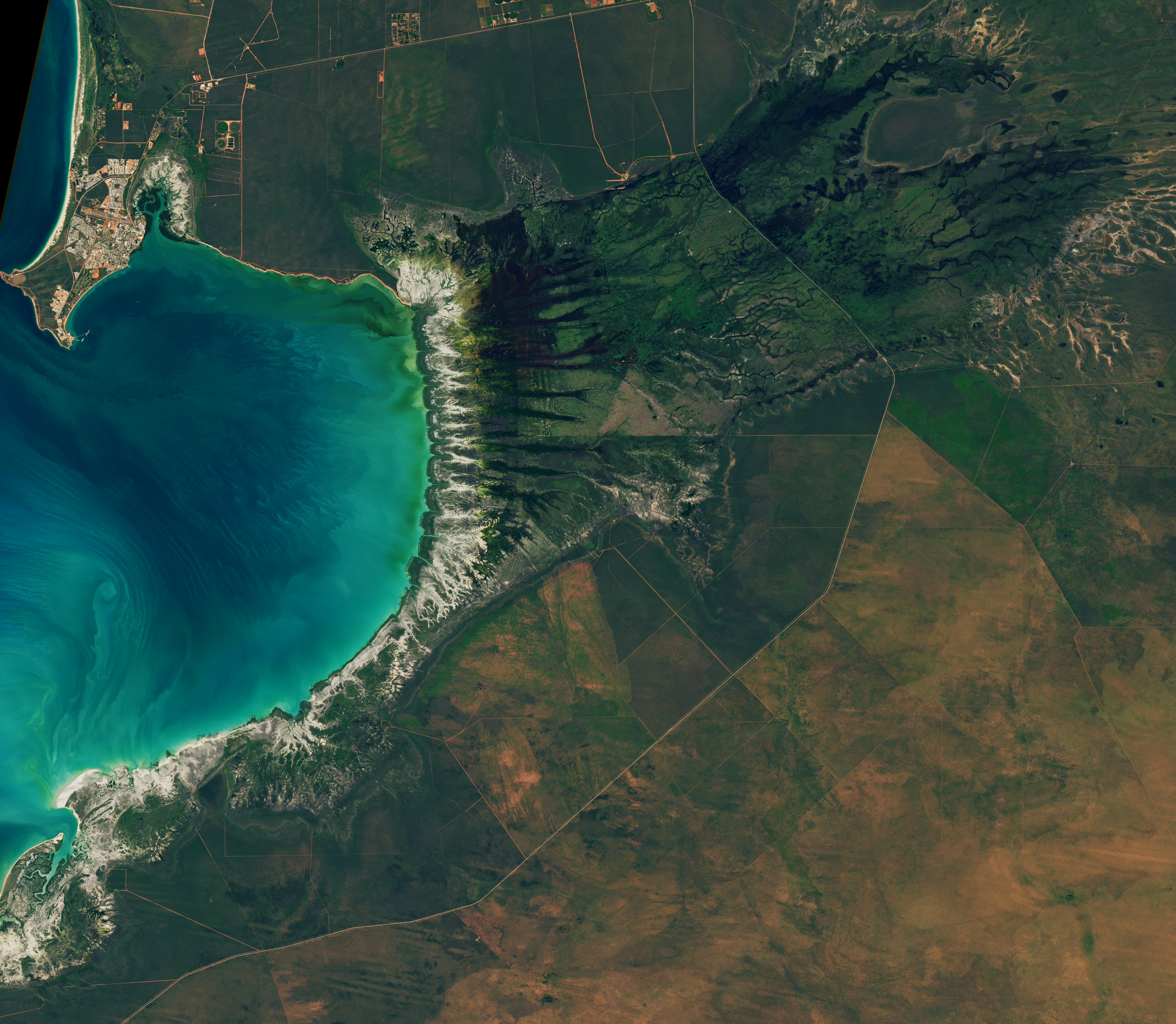
The image at the top of the page shows the bay on March 18, 2026, when water levels were high. Green mangrove forests grow thickly along the shoreline and line the mouths of a network of evenly spaced, linear tidal creeks. These mangrove forests are dynamic. Analysis of decades of Landsat observations shows them expanding westward by nearly 2 meters per year as sediment from the waterways to the east accumulates in the sheltered bay.
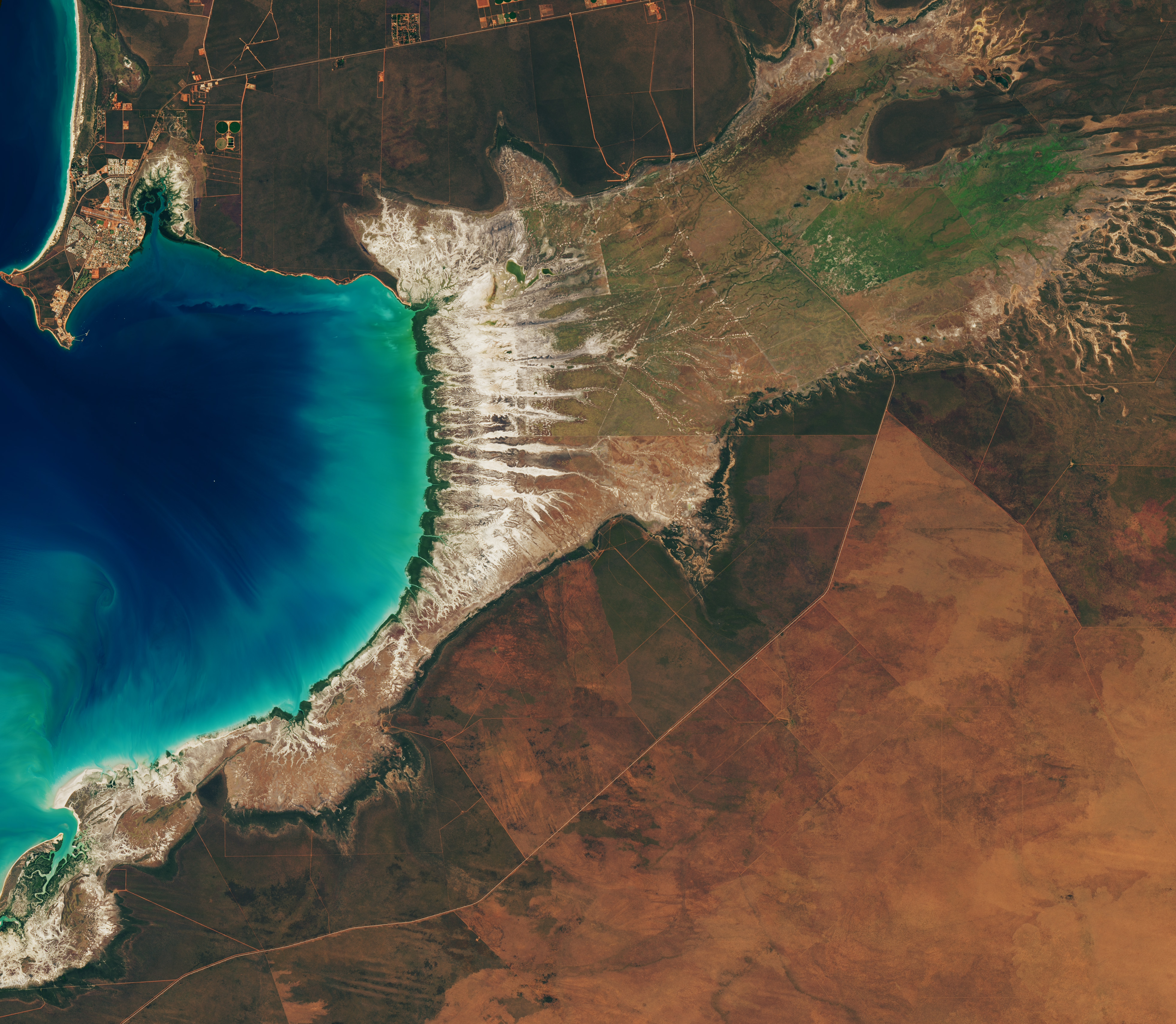
Farther inland, branching networks of tidal drainage channels connect with the tidal creeks, giving the bay its feathered appearance. These channels, partially obscured by thick vegetation in March, were more visible earlier and later in the year, when vegetation was thinner.
Around Roebuck Bay, inland vegetation greens after monsoon rains, peaking in March, and turns brown and dry by June. The Landsat 8 and 9 satellites captured these images throughout 2026.
NASA Earth Observatory / Lauren Dauphin
Monsoonal rains, typically falling between December and March, transform the landscape around the bay into lush grasslands and seasonal wetlands. As the rains fade in May and June and the dry season takes hold, these ephemeral grasses and sedge ecosystems die back, turning the landscape shades of gold and brown. The consistent spacing of the tidal creeks is likely not a tidal effect; it appears to be influenced by the regular spacing of linear dunes in the broader region, as seen in the plains to the east.
The bay’s dramatic tidal and seasonal changes are striking from above, and they also support a bounty of life on the ground. The mangroves serve as nurseries for crustaceans and fish, and the mudflats teem with dozens of types of invertebrates, including snails, worms, crabs, clams, and cockles. Shells and snails can reach an abundance of 2,500 per square meter, according to the Australian government.
This bounty of marine life is a major draw for birds. The bay, one of the most important sites for migratory birds in Australia and a key stop on the East Asian-Australasian Flyway, regularly hosts hundreds of thousands of birds, including plovers, godwits, and knots.
NASA Earth Observatory images by Lauren Dauphin, using Landsat data from the U.S. Geological Survey.Story by Adam Voiland.
Downloads
January 29, 2026
JPEG (3.65 MB)
March 18, 2026
JPEG (3.41 MB)
June 20, 2026
JPEG (3.61 MB)
References & Resources
Birdlife International (2026) Roebuck Bay. Accessed August 10, 2026.
Brockmann Consult (2025) Roebuck Bay. Accessed August 10, 2026.
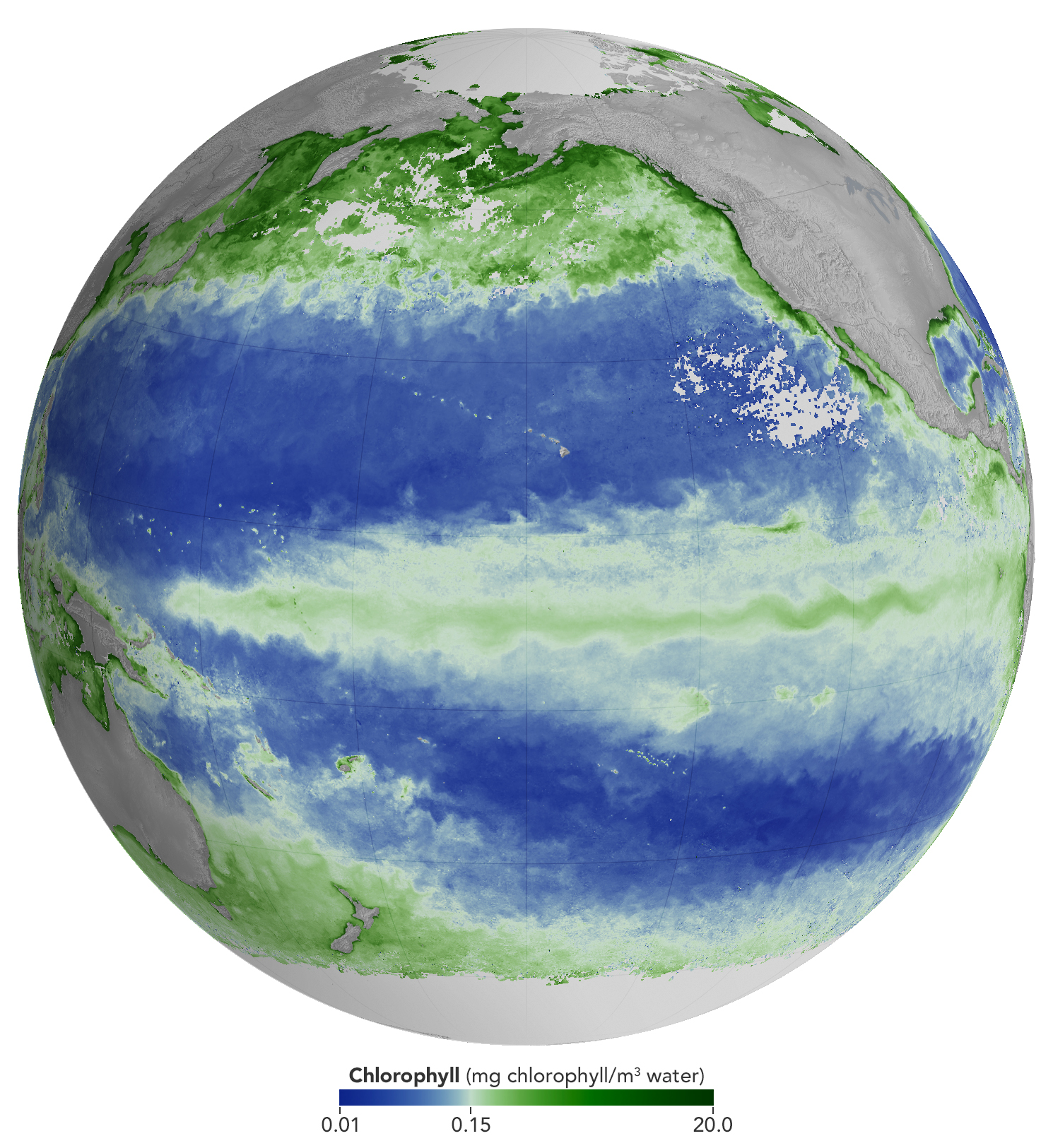
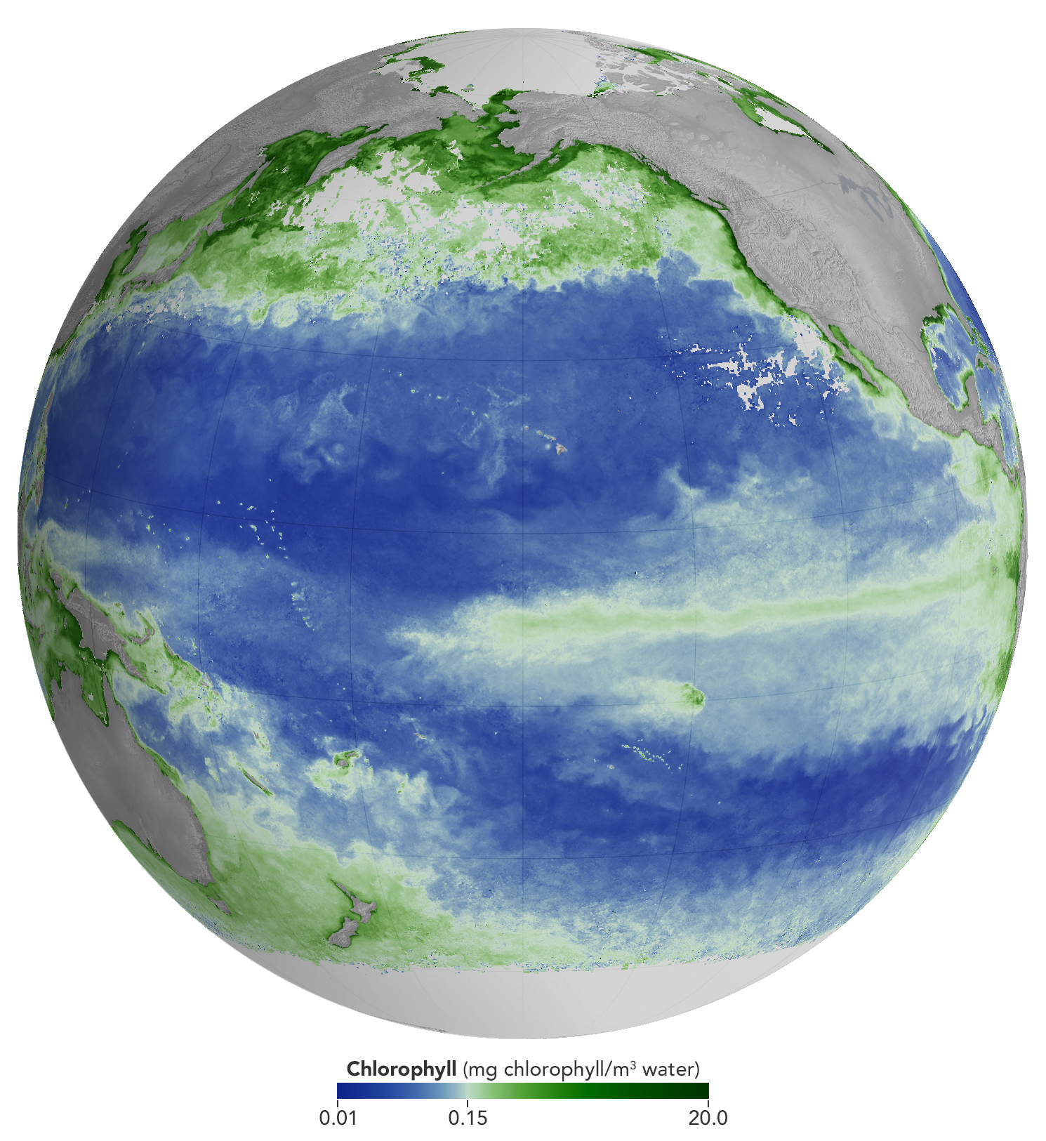
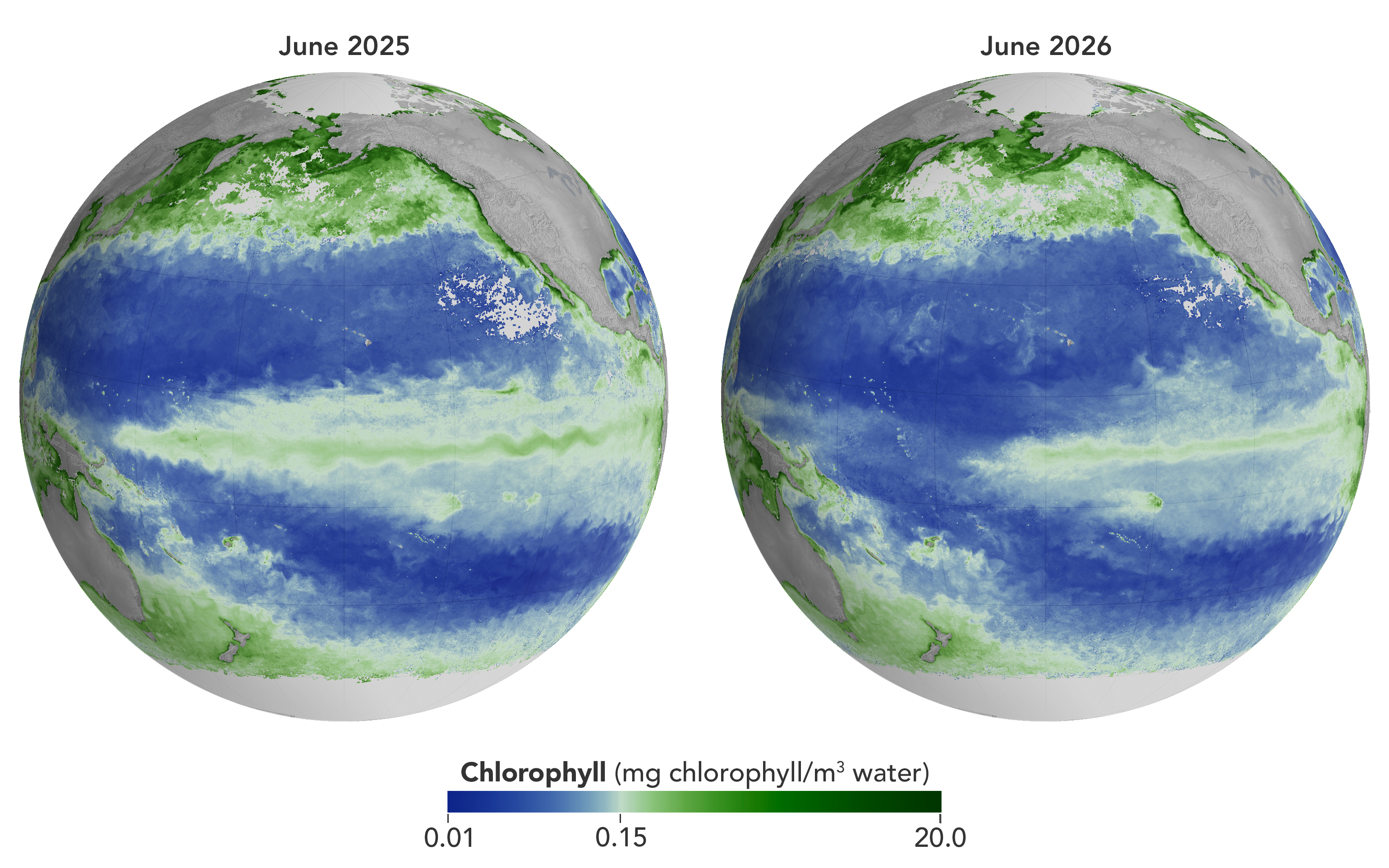
Concentrations of chlorophyll in the equatorial Pacific deviate from normal during El Niño events. These maps depict monthly average chlorophyll concentrations for June 2025 (left), under neutral conditions, and June 2026 (right), as El Niño was strengthening. Data come from the OCI (Ocean Color Instrument) on NASA’s PACE (Plankton, Aerosol, Cloud, ocean Ecosystem) satellite and are based on measurements of green and blue light from the ocean reflected back to the sensor. NASA Earth Observatory images by Michala Garrison.
As of June 2026, El Niño has officially arrived. This naturally recurring phenomenon is characterized by warmer-than-normal water temperatures in parts of the equatorial Pacific along with changes to atmospheric and oceanic circulation patterns. Its regional effects range from desert floods to delayed monsoons to shifts in where tropical cyclones are more likely to form.
NOAA’s Climate Prediction Center expects the current El Niño to continue to strengthen through the end of 2026, with a 97 percent chance of lasting through early Northern Hemisphere spring 2027. Even during El Niño’s early stages, satellites have observed characteristic changes along the equatorial Pacific, such as warmer-than-normal sea surface temperatures and higher-than-normal sea surface height.
Among the first ecological downstream effects are changes to the marine food web. The maps above show chlorophyll-a concentrations—the pigment present in most phytoplankton—as observed by the OCI (Ocean Color Instrument) on NASA’s PACE (Plankton, Aerosol, Cloud, ocean Ecosystem) satellite. In June 2025 (left), conditions were neutral, while in June 2026 (right), El Niño was strengthening.
The most noticeable difference appears in the central Pacific, around the equator due north of New Zealand: chlorophyll concentrations, an indication of phytoplankton abundance, are substantially lower in 2026. This change is expected, said Matthew Kehrli and Graham Trolley, oceanographers in the Ocean Ecology Laboratory at NASA’s Goddard Space Flight Center. That’s because during an El Niño, easterly equatorial trade winds weaken, the warm surface layer of the ocean extends deeper, and the upwelling of cool, nutrient-rich water that typically fuels phytoplankton growth is suppressed.
As the El Niño progresses, the scientists anticipate the differences in the central Pacific will become more pronounced. “This may manifest as a greater difference in values across the current region, as a broadening region of reduced surface chlorophyll-a concentration, or both, depending on the behavior of the equatorial trade winds,” they said.
Reductions in phytoplankton have ripple effects through the marine food web, including in coastal regions. Less food is available for zooplankton, as well as for fish, seabirds, and marine mammals. Peru’s anchovy fisheries have seen profound declines in catch during past El Niños, driven similarly by warmer surface waters, reduced upwelling, and lower phytoplankton abundance. In 2026, Peru’s Ministry of Production repeatedly suspended the fishery to safeguard the country’s main fishing resource. Pelicans have been seen venturing into Peruvian ports and urban areas in search of food.
Although the disruptions to marine life can be severe, a post-El Niño “chlorophyll rebound,” with higher-than-normal concentrations in the equatorial Pacific, can occur. Research suggests that higher iron concentrations delivered in ocean currents, as well as dust arriving from drier land in parts of Central and South America, help fuel the resurgence—a rebound that doesn’t require a follow-on La Niña. La Niña, which often follows El Niño events, can also produce elevated chlorophyll concentrations. A strong La Niña in 1998–1999 set off a large phytoplankton bloom in the eastern Pacific and a dramatic increase in fish populations.
Scientists have new tools available for studying this sort of variability. The PACE mission launched in February 2024, making this the first complete El Niño event for which the satellite will gather global, near-daily hyperspectral measurements. “The scientific community will be able to observe the 2026 El Niño with data across more wavelengths of light than ever before,” Kehrli and Trolley said.
To better understand effects on life in the ocean, researchers hope to use PACE data to gauge the responses of specific phytoplankton communities to El Niño. And the possibilities extend beyond the marine realm, the scientists note. PACE’s sensors can measure plant pigment composition on land and clouds and aerosols in the atmosphere, all of which are influenced by El Niño.
Surface temperatures across Earth’s poles pulse with the seasons, as seen in this animation based on two years of data collected by NASA’s PREFIRE (Polar Radiant Energy in the Far-InfraRed Experiment) mission.
NASA/Chad Greene
At the top and bottom of the planet, the seasons arrive on a schedule all their own. Satellite data from a mission measuring infrared energy reveal just how differently—and how dramatically—surface temperatures swing across two full years at the poles.
In this animation, surface temperatures across the Arctic and Antarctic pulse between cold (dark blue) and milder to warm (lighter blue to red). Data for the animation come from NASA’s PREFIRE (Polar Radiant Energy in the Far-InfraRed Experiment) satellites. The mission’s twin CubeSats began collecting science data in July 2024 and have now captured two complete seasonal cycles at each pole.
Because the two poles sit in opposite hemispheres, their seasons occur at opposite times—and the swing between seasons differs, too. In the Arctic, cold, dark winters give way to summers warm enough to thaw vast stretches of tundra and sea ice. In Antarctica, Earth’s coldest continent, summer temperatures rarely climb above freezing before the bitter cold of winter returns.
Surface temperatures, and how they fluctuate, offer a window into Earth’s energy budget, the net flow of energy into and out of the Earth system. Sunlight absorbed by the surface is re-radiated as infrared heat, which bounces between Earth’s surface and atmosphere before escaping to space. The poles play an important role in this process. Atmospheric and ocean circulation carries excess heat absorbed in the tropics toward the poles, where it radiates away to space, helping regulate the planet’s temperature.
“By measuring invisible heat radiating from Earth’s coldest places, PREFIRE is helping scientists understand why the poles are changing so rapidly, and what those changes might mean for the rest of the planet,” said Chad Greene, a glaciologist at NASA’s Jet Propulsion Laboratory.
Scientists have long known that far-infrared radiation accounts for nearly 60 percent of the energy Earth loses to space, but that portion of the spectrum—invisible to human eyes—had never been comprehensively measured on a global scale. By directly tracking this invisible energy in near-real-time, the PREFIRE mission is helping scientists refine models and gain a better understanding of the Earth system.
“Weather systems, river flows, shipping routes, and ice sheet stability are all influenced by energy movement in a part of the spectrum that only PREFIRE can see,” said Tristan L’Ecuyer, an atmospheric scientist at the University of Wisconsin-Madison and principal investigator of the PREFIRE mission. “Now that the invisible has been made visible, we can begin to improve weather and climate predictions that industries, our national defense, and Arctic communities rely on.”
Maps courtesy of Chad Greene, NASA/JPL, using data from NASA’s PREFIRE mission. Story by Kathryn Hansen.
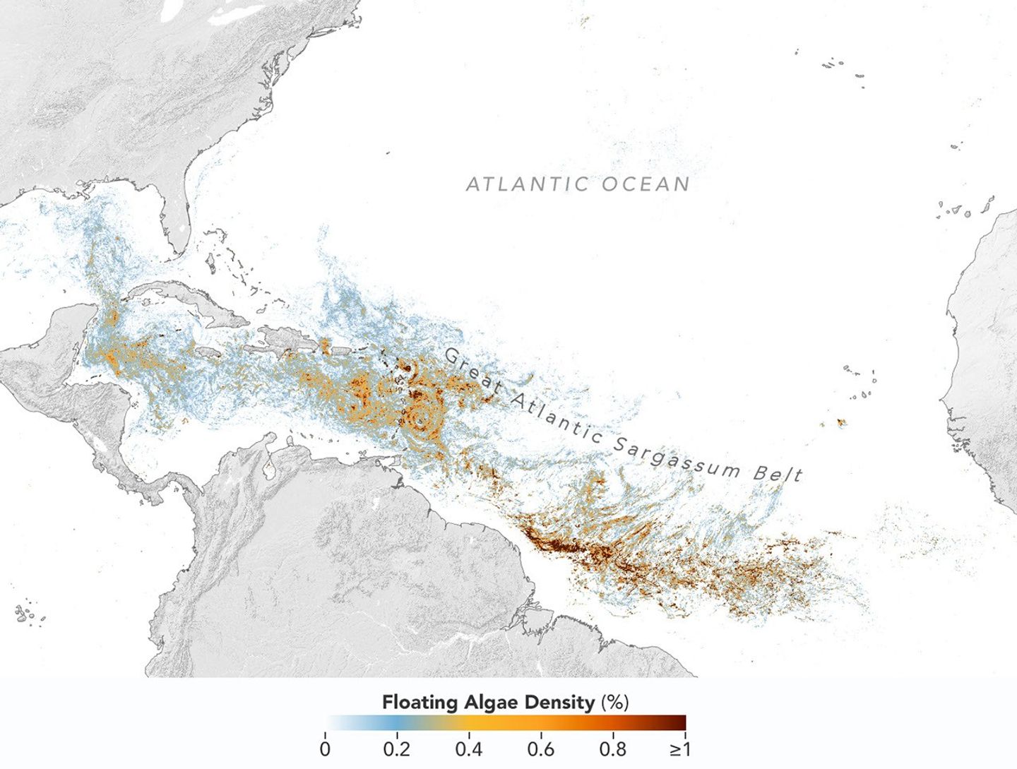
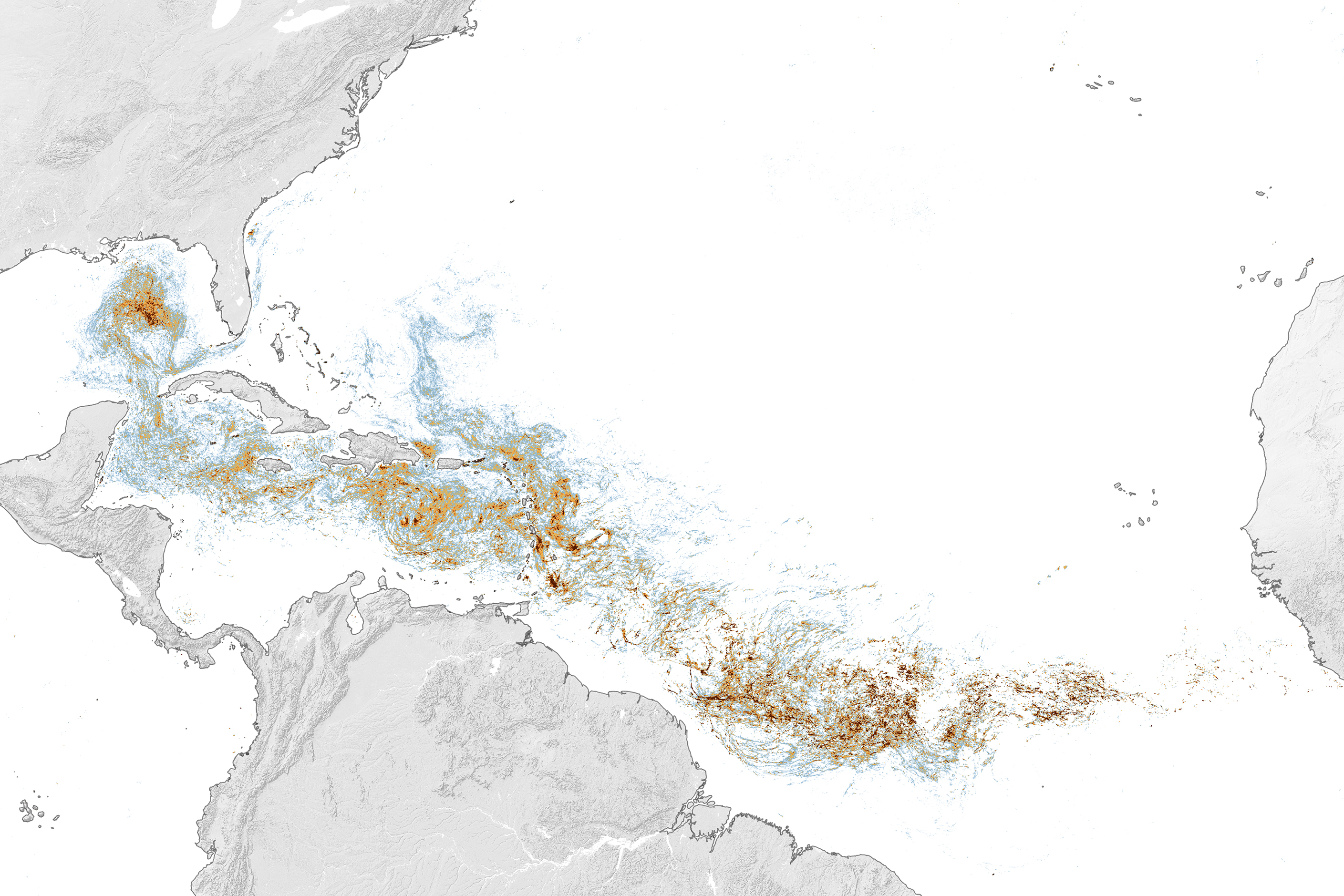
This map, based on data from the OCI (Ocean Color Instrument) on NASA’s PACE (Plankton, Aerosol, Cloud, ocean Ecosystem) satellite, shows Sargassum highly concentrated in the tropical Atlantic in June 2026.
NASA Earth Observatory/Lauren Dauphin
Sargassum, a type of brown floating algae, has shifted its range in recent decades, thinning out in the North Atlantic’s Sargasso Sea while proliferating in the tropical Atlantic. That trend, underway since 2011, continued in 2026 as the algae, commonly known as a type of seaweed, reached its annual peak in June across a stretch of ocean known as the Great Atlantic Sargassum Belt.
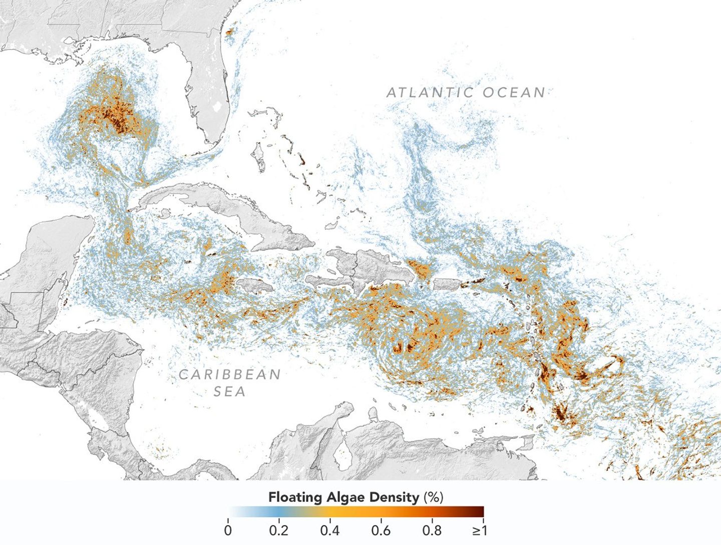
The belt’s Sargassum abundance in June 2026 made it the second-highest Sargassum year in the satellite record, slightly behind 2025, according to scientists at the University of South Florida (USF) College of Marine Science. Regionally, the Caribbean Sea and the Gulf of America (Gulf of Mexico) both hit record highs, according to USF’s June 2026Sargassum outlook. The western and eastern Caribbean saw 3.6 and 9 million metric tons, respectively, while the Gulf saw 5 million metric tons—nearly double its previous record, also set in 2025.
“The belt is a basin-scale phenomenon that can have devastating local-scale impacts throughout the Caribbean and Gulf, and satellite observations are the only method that captures both scales on a daily basis,” said Brian Barnes, a marine scientist at the Optical Oceanography Laboratory at USF. “The tracking done by our lab helps communities know the current extent of Sargassum and prepare for what’s to come.”
In moderate amounts in the open ocean, Sargassum provides habitat for turtles, invertebrates, fish, and birds, and adds oxygen to the water through photosynthesis. But too much of it near shore can tangle and suffocate marine life, and mats that sink can smother corals and seagrasses. On beaches, decomposing Sargassum releases hydrogen sulfide, a rotten-egg-smelling gas that’s a potential problem for both ecosystems and tourism.
The map above shows Sargassum density in the tropical Atlantic Ocean in June 2026. Red and orange areas are where Sargassum densities were the highest. Note that although the “belt” appears continuous, discrete Sargassum mats are scattered across the ocean surface. The map is based on satellite measurements of how much of the ocean surface was covered by the seaweed, averaged per pixel across all observations made in June by the OCI (Ocean Color Instrument) on NASA’s PACE (Plankton, Aerosol, Cloud, ocean Ecosystem) satellite.
This detailed view of the same PACEOCI map highlights Sargassum concentrations across the Caribbean Sea and Gulf of America, both of which saw record-high amounts of the floating algae in June 2026.
NASA Earth Observatory/Lauren Dauphin
Ocean currents and winds shape the Sargassum belt, which, despite the patchiness, stretches nearly continuously from West Africa to the Gulf and holds a fairly steady “width” from the western tropical Atlantic westward, explained Chuanmin Hu, also an optical oceanographer at USF. The ocean currents have also spared Florida’s west coast from inundation this summer, while delivering large amounts of seaweed to the Florida Keys and the state’s east coast. The bulk of the Sargassum, however, is visible in the Caribbean Sea, shown in detail above, where problems associated with inundation have been more severe, Hu said.
Data for the maps were provided by Lin Qi, an oceanographer at NOAA’s Center for Satellite Applications and Research, who has been working to generate Sargassum maps based on data from PACE, which was launched in February 2024. The work extends that of Qi and colleagues at USF’s Optical Oceanography Laboratory. This team first developed Sargassum detection techniques using MODIS (Moderate Resolution Imaging Spectroradiometer) on NASA’s long-running Terra and Aqua satellites and VIIRS (Visible Infrared Imaging Radiometer Suite) on the NOAA-20 satellite—data that have been a key component of USF’s Sargassum Watch System and of research into the seaweed’s longer-term trends.
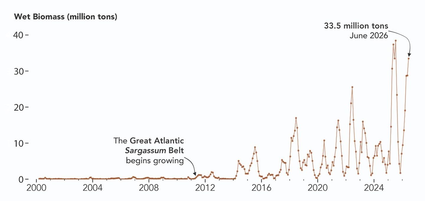
Satellites detect Sargassum by its signals in reflected sunlight. Because of its plant structure and chlorophyll pigments, Sargassum reflects more near-infrared light than water. Scientists flag pixels where the reflectance spikes above the levels produced by plain seawater, and then they use the strength of this spike to estimate Sargassum density, which refers to the fraction of ocean surface covered by the seaweed in each pixel. Density estimates can then be converted into biomass, or the total weight of Sargassum present within a pixel, which is how the longer-term trends in the chart below are tracked.
NASA Earth Observatory/Lauren Dauphin
The chart above uses the continuous MODIS record since March 2000 to show how Sargassum biomass across the Great Atlantic Sargassum Belt has changed through June 2026. Notice the uptick beginning around 2011, when the belt was first developing, and the seasonal dips in winter and peaks in spring and summer. The record high in July 2025 stands out, followed by the quick rise in early 2026—especially in the first four months of the year—that culminated in the year’s peak in June. More recent observations, not yet reflected in the chart, indicate Sargassum biomass declined through the following month of July.
“Since the initial appearance of the Great Atlantic Sargassum Belt in 2011, the total Sargassum amount in the Atlantic Ocean has increased substantially, more than doubling every five years,” Hu said. He added that the exact mechanism is still being investigated, but it’s possibly related to ocean warming, multiple nutrient sources, and the fact that large Sargassum mats attract other organisms—such as nitrogen-fixing bacteria—that can supply additional nutrients to sustain further growth.
Alongside data from MODIS and VIIRS, OCI data from PACE now feeds into the Sargassum Watch System’s near-real-time daily and weekly composite maps. A recent study of the central-west Atlantic led by Qi, spanning May through August 2024, found that OCI offers several advantages over its predecessors, observing more of the ocean and detecting Sargassum with greater sensitivity.
Hu noted that the added pixels from OCI can improve near-real-time monitoring and analyses of short-term fluctuations. And its higher sensitivity, he said, will also lead to improved maps during winter months, “thus helping understand Sargassum changes over time.”
Additionally, the study’s authors found that OCI’s hyperspectral capability makes it the only sensor able to spectrally discriminate Sargassum pixels across the Atlantic Ocean “without ambiguity,” adding confidence to the interpretation of detected image features—especially in parts of the Atlantic where another type of floating algae, Trichodesmium, has been reported.
“I think I can speak for all project members, past and present, in sharing how rewarding it is to see the promise of PACE’s advancements come to life,” said Jeremy Werdell, PACE project scientist at NASA’s Goddard Space Flight Center. “OCI has started a true renaissance in aquatic ecosystem monitoring from space.”
NASA Earth Observatory maps and chart by Lauren Dauphin, using PACE and MODIS data courtesy of Lin Qi (NOAA), and Brian Barnes and Chuanmin Hu (University of South Florida, Optical Oceanography Laboratory). Story by Kathryn Hansen.
Smoke pours from dozens of large fires in Oregon in this image captured by MODIS (Moderate Resolution Imaging Spectroradiometer) on NASA’s Aqua satellite on July 26, 2026.
NASA Earth Observatory/Michala Garrison
Dry thunderstorms that popped up over the Cascade Range on the evening of July 15, 2026, peppered Oregon and Washington with thousands of lightning strikes as they moved east across the states. By the following day, NASA satellites had begun to detect large numbers of wildland fires burning throughout central and eastern Oregon.
Though initially small, these blazes strengthened as they were fanned by gusty winds and raced through landscapes parched by extreme drought and baking in summer heat. When NASA’s Aqua satellite captured the image shown above on the afternoon of July 26, smoke poured northeast from dozens of large fires that had collectively charred hundreds of square miles. The fires produced a blanket of haze, prompting state officials to issue air quality advisories for eastern Oregon.
Many communities faced evacuation orders as more than 10,000 firefighters battled wildfires throughout the state. On the day the image was captured, the largest active fires were the Hay Creek Complex, Brewer, Big Grass, Akawa Butte, and Powder River fires. Several of these blazes were less than 5 percent contained, according to the National Interagency Fire Center. State officials invoked Oregon’s Emergency Conflagration Act to protect communities as they responded to particularly threatening fires such as the Shingle, Bench, Beachcomb, and Second Flat fires.
Government satellite data are part of a global system of observations used to track fire behavior and analyze emerging trends. Among the real-time wildfire monitoring tools that NASA makes available are FIRMS (Fire Information for Resource Management System), the Worldview browser, and the Fire Event Explorer.
As of July 27, 2026, fires in Oregon had burned more than one million acres, according to news outlets. Meanwhile, the National Interagency Fire Center reported that fires had burned more than 4 million acres across the United States. The 10-year average (2016-2025) for this point in the season is 3.4 million acres.
NASA Earth Observatory image by Michala Garrison, using MODIS data from NASA EOSDIS LANCE and GIBS/Worldview.Story by Adam Voiland.
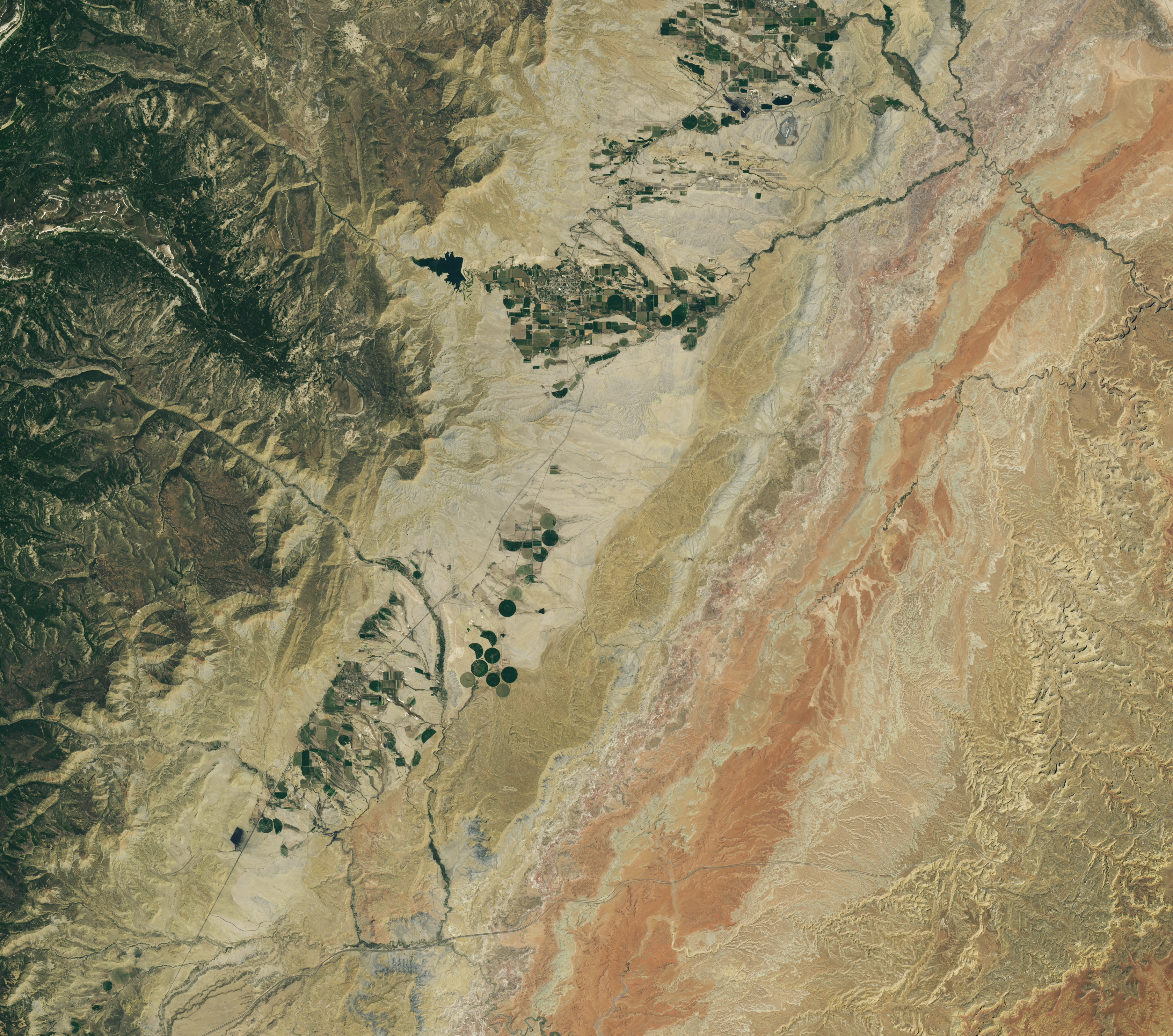
A dry, tan-colored valley containing a few circular irrigated fields runs roughly north-south through the image.
NASA Earth Observatory / Lauren Dauphin
Grid-like arrays of solar panels cover parts of a valley floor in a brown, dry-looking area of Utah.
NASA Earth Observatory / Lauren Dauphin
A dry, tan-colored valley containing a few circular irrigated fields runs roughly north-south through the image.
NASA Earth Observatory / Lauren Dauphin
Grid-like arrays of solar panels cover parts of a valley floor in a brown, dry-looking area of Utah.
NASA Earth Observatory / Lauren Dauphin
June 16, 2024
June 6, 2026
The nearly one million photovoltaic panels of a solar energy and battery storage facility in Utah appear in the right image, acquired with the OLI (Operational Land Imager) on Landsat 8 on June 6, 2026. The same sensor captured the left image on June 16, 2024. NASA Earth Observatory images by Lauren Dauphin.
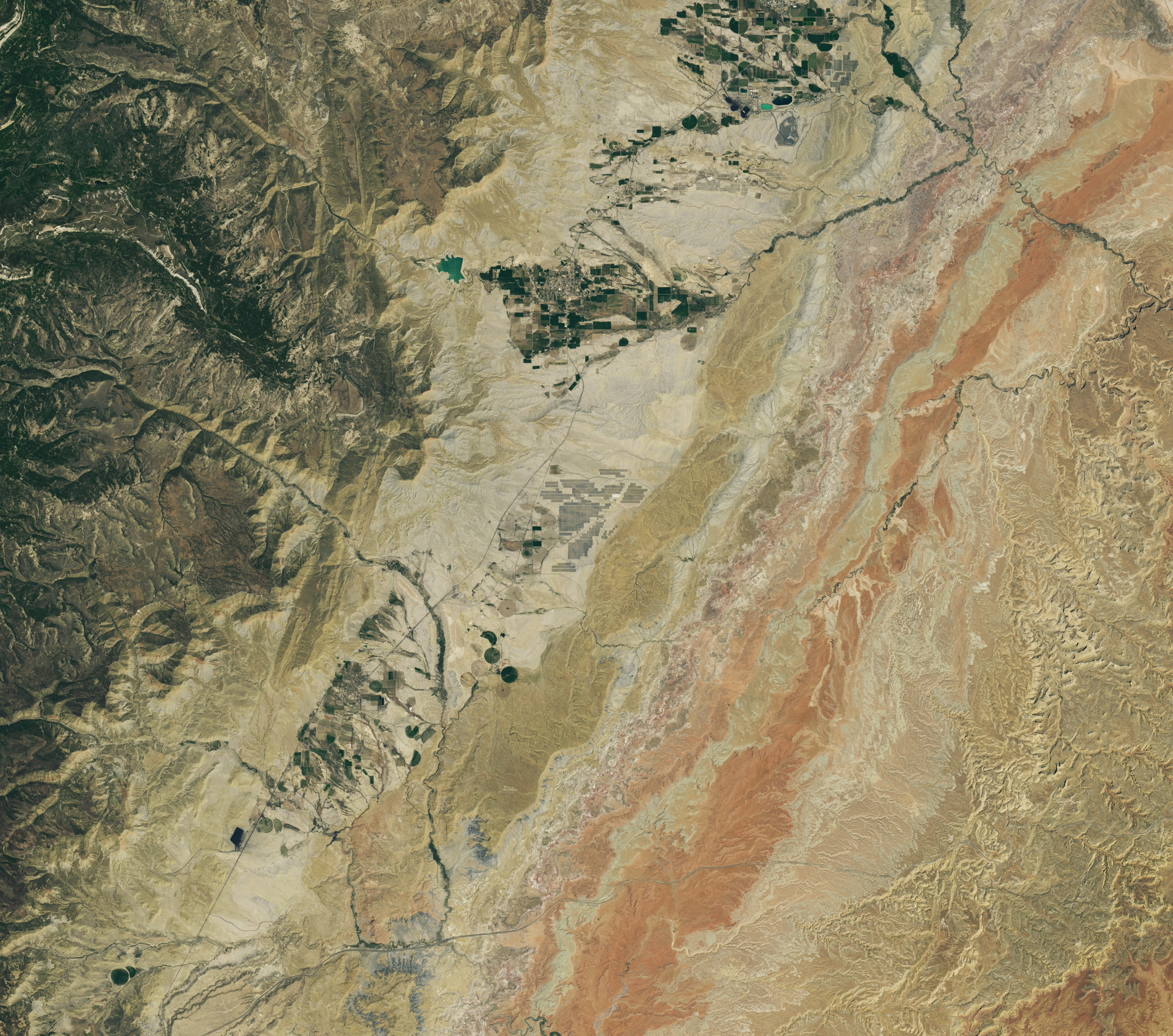
Historically, central Utah’s Castle Valley has been a coal hub, with mining operations on the slopes of the Wasatch Plateau to the west active since the late 1800s. A different energy development arrived in the region in June 2026, when a large solar power and battery storage plant came online in the sunny valley about 130 miles (210 kilometers) southeast of Salt Lake City.
The recently constructed Green River Energy Center, seen in the Landsat 8 image above (right), features nearly one million solar panels and roughly 500 batteries on several square miles of previously undeveloped land. The facility has 400 megawatts of solar-generating capacity with another 400 megawatts of battery storage. That places it among the many utility-scale solar power and battery storage projects that the U.S. Energy Information Administration expects to be plugged into the country’s grid in 2026.
The Utah facility is slated to supply power to Salt Lake City and other areas across the state, according to news reports, and project staff estimate it could produce enough electricity for more than 100,000 homes. With its integrated battery storage, the plant has the potential to generate power at all hours, even when the Sun isn’t shining. And the Green River Energy Center can build on Castle Valley’s energy legacy by utilizing existing transmission lines originally built for coal-fired power plants in the area.
Though Utah adopted coal as its state rock and has long relied on it for energy, other sources, such as solar and geothermal, are becoming larger parts of the state’s energy mix. In 2025, coal fueled about half of the state’s electricity generation, down from about 75 percent in 2015. Meanwhile, solar grew to account for about 14 percent of generation in 2025, up from nearly zero a decade before. Satellite data can be useful to planners and policymakers involved in energy transitions for assessing the potential of renewable energy systems and tracking their adoption and performance.
NASA Earth Observatory images by Lauren Dauphin, using Landsat data from the U.S. Geological Survey. Story by Lindsey Doermann.
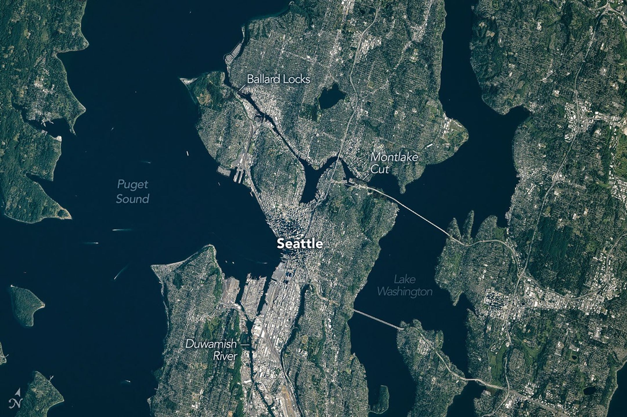
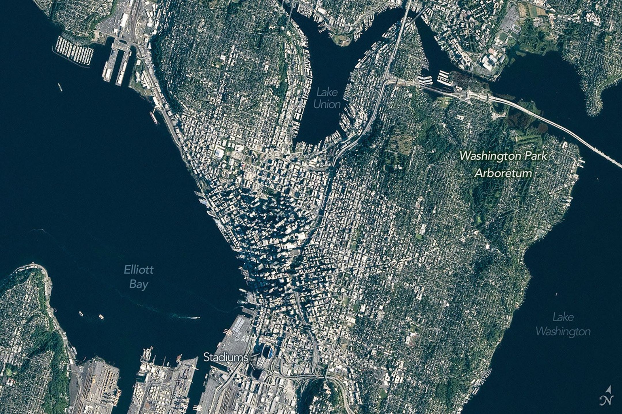
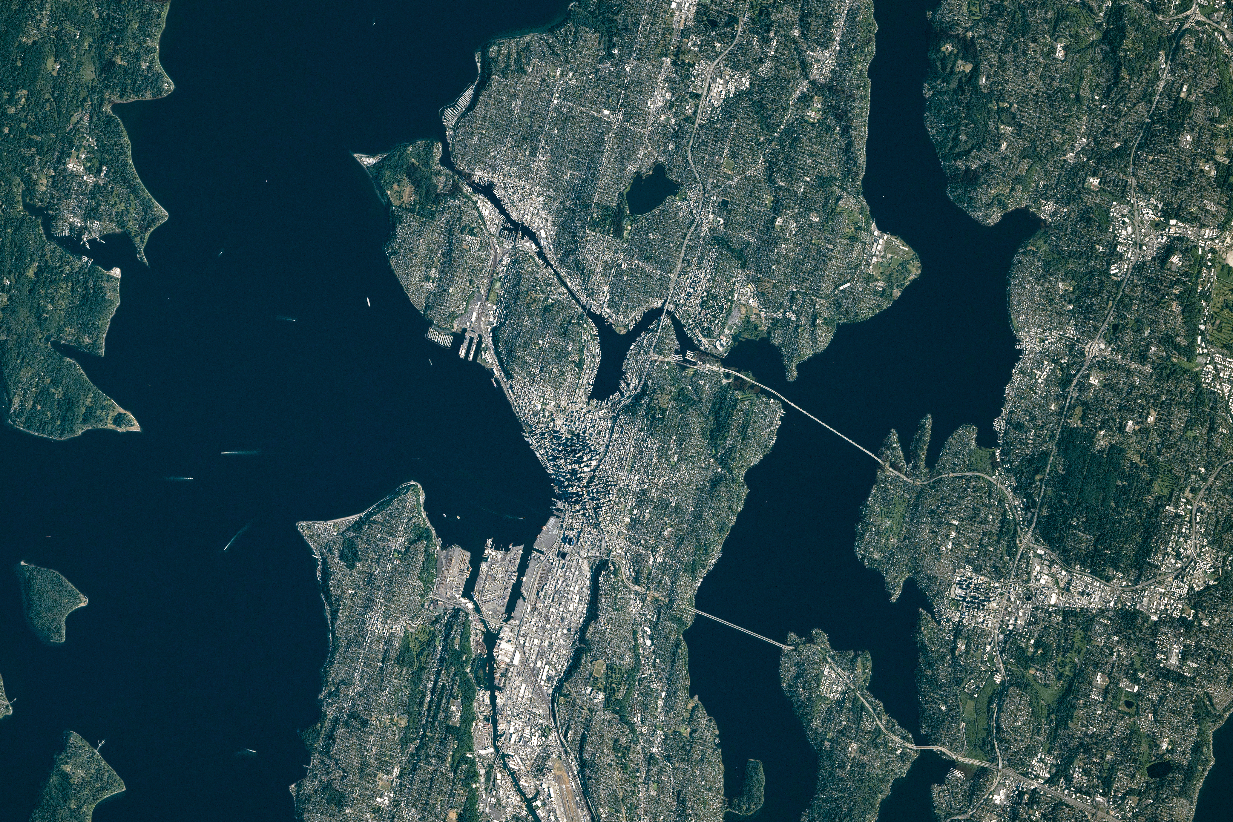
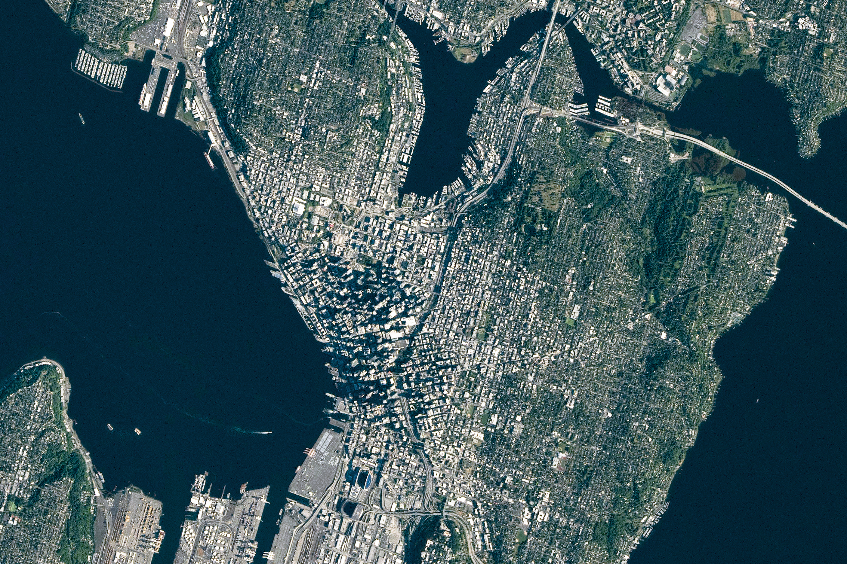
Seattle, Washington—sometimes known as the “Emerald City”—was glimmering in the morning sunlight when an astronaut aboard the International Space Station took this photo on June 16, 2026. The city’s parks and tree-filled neighborhoods lend a lush, green look to the metropolis, while tall buildings downtown cast long shadows and ships navigate surrounding waterways.
The broad contours of the city’s landscape and the water around it owe their shape to the advance and retreat of glaciers during the last ice age. Between roughly 18,000 and 16,000 years ago, the Puget lobe of the Cordilleran ice sheet covered the area in a mass of ice up to 3,300 feet (1,000 meters) thick. The glacier scoured the basins now occupied by Puget Sound and the region’s lakes.
The glacier left its mark above water, too. Several of Seattle’s notorious hills (of which there are seven or more, depending on who’s counting) are drumlins. These elongated mounds of glacial debris run north-south, parallel to the direction of the ice’s movement. East-west travelers in the city, facing challenging ups and downs, may attest to this topographic trend.
The ice also transported large boulders called glacial erratics from more northerly locations and deposited them around the region. A particularly large erratic, the Wedgwood Rock, stands about 20 feet (6 meters) tall and draws its name from the North Seattle neighborhood in which it rests.
June 16, 2026
In more recent times, humans have undertaken projects to rework the topography. Notable alterations include leveling Denny Hill north of downtown and filling in tideflats at the mouth of the Duwamish River south of downtown, which created around 1,300 acres of new land. Seattle’s professional sports stadiums sit atop this fill.
This photo was acquired after several development projects to update waterfront infrastructure downtown, initiated in 2010, were completed. These include a new ferry dock and terminal, a rebuilt seawall, and a tunnel to replace an above-ground highway and create more inviting public access to the waterfront.
Some replumbing of the region’s waterways is apparent from the astronaut’s perspective, as well. In the 1910s, the Army Corps of Engineers built canals on either side of Lake Union to connect Puget Sound (an inlet of the Pacific Ocean) with Lake Washington. Starting in 1916, the Montlake Cut connected Lake Washington to Lake Union, and the Ballard Locks, northwest of Lake Union, began raising and lowering watercraft between the freshwater lakes and tidal Puget Sound. As a result of this project, Lake Washington’s water level dropped about 9 feet (3 meters) and ceased draining from its natural outlet at its southern end.
Today, the waters in and around Seattle support many uses: container ships, cruise ships, car and passenger ferries, floatplanes, and recreational craft ply the sound and lakes. And as for Seattle’s emerald nickname, pockets of old-growth forest still exist within city limits, containing centuries-old trees such as Douglas fir, Western red cedar, and Western hemlock. Seattleites often spot wildlife such as bald eagles, coyotes, and sea lions in the city’s various habitats.
Astronaut photograph ISS074-E-723719 was acquired on June 16, 2026, with a Nikon Z9 digital camera using a focal length of 560 millimeters. It is provided by the ISS Crew Earth Observations Facility and the Earth Science and Remote Sensing Unit at NASA Johnson Space Center. The image was taken by a member of the Expedition 74 crew. The image has been cropped and enhanced to improve contrast, and lens artifacts have been removed. The International Space Station Program supports the laboratory as part of the ISS National Lab to help astronauts take pictures of Earth that will be of the greatest value to scientists and the public, and to make those images freely available on the Internet. Additional images taken by astronauts and cosmonauts can be viewed at the NASA/JSC Gateway to Astronaut Photography of Earth. Story by Lindsey Doermann.
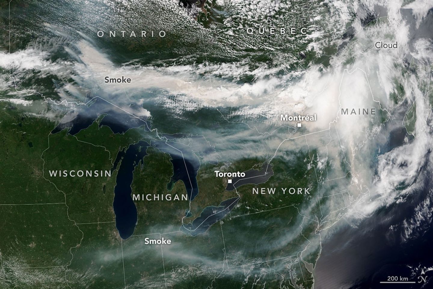
Smoke from wildland fires pours eastward over Canada and the U.S. in an image captured on the afternoon of July 14, 2026, by the VIIRS (Visible Infrared Imaging Radiometer Suite) on the NOAA-21 satellite.
NASA Earth Observatory/Lauren Dauphin
After a slow start to Canada’s 2026 fire season, activity picked up by the end of June amid dry, warm conditions and returned closer to the 25-year average. By mid-July, almost 850 fires were actively burning across the country, according to the Canadian Interagency Forest Fire Centre. More than 180 of those were burning in Ontario.
This NOAA-21 image, acquired on the afternoon of July 14, 2026, shows smoke billowing from the Ontario fires. Winds carried the smoke primarily southeast over much of the southern part of the province, as well as parts of Quebec and the U.S. Midwest and Northeast, tinting the sky shades of gray and yellow and the Sun orange in many areas.
The smoke’s impact on air quality varied, depending largely on altitude. In areas where smoke was high in the atmosphere, air quality impacts were negligible; where it drifted closer to the ground, conditions worsened. Air quality in Toronto, for instance, reached unhealthy levels, according to AirNow. People in the southern parts of the province were also grappling with a heat wave, compounding the health risks.
Much of the smoke came from fires in Northwestern Ontario, where eight blazes saw significant growth on July 13 and 14. The fires prompted officials to issue evacuation orders for several communities in this part of the province, according to news reports.
As of July 14, fires across Canada have burned 1.9 million hectares (4.7 million acres) since the start of the year—still well below the season totals from the extreme fire years of 2023 and 2025. How the rest of the season plays out remains to be seen. A seasonal fire outlook—compiled by wildland fire experts from the U.S., Canada, and Mexico—shows where fire conditions are more or less likely through July, August, and September.
NASA Earth Observatory image by Lauren Dauphin, using VIIRS data from NASA EOSDIS LANCE , GIBS/Worldview , and the Joint Polar Satellite System (JPSS). Story by Kathryn Hansen.
Downloads
July 14, 2026
JPEG (3.96 MB)
References & Resources
AirNow (2026, July 15) Wildfires. Accessed July 15, 2026.

 Login