❌

Normal view

Finishing Off an Asteroid

7 August 2026 at 17:00

A rendering of a small star surrounded by a ring of gas and some larger asteroids.

Only one white dwarf star has ever been caught eating an asteroid. Recently, however, astronomers may have found another that just finished its meal.

Eating Asteroids

Although stars like our Sun don’t explode in violent supernovae like their massive counterparts, they don’t slink quietly into a peaceful old age either. When a solar-mass star reaches the end of its main sequence life, it first swells dramatically (the Sun may eventually grow so large that it consumes Earth and the device you’re reading this on), then shrinks down to a tiny but incredibly hot ember known as a white dwarf.

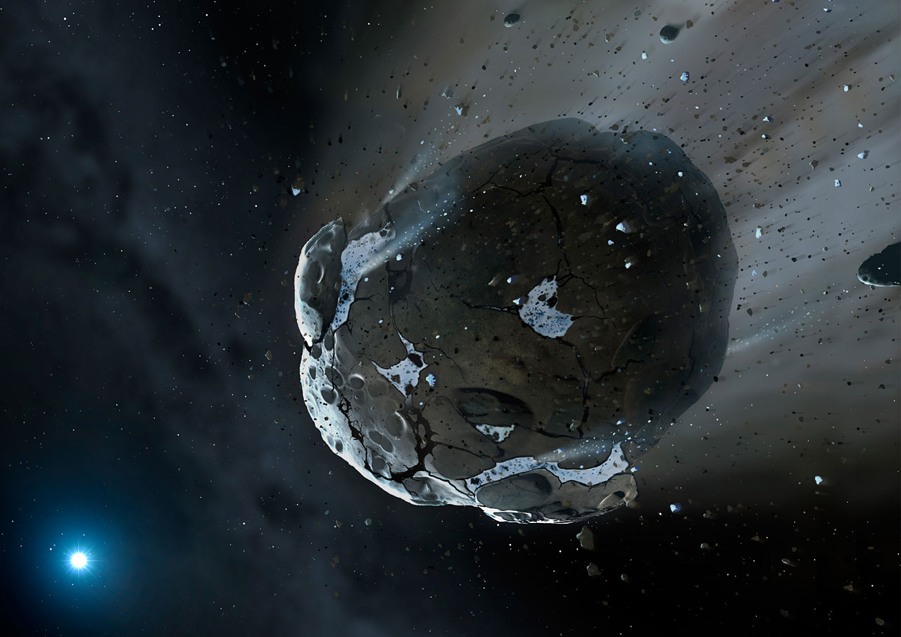
A rendering of an asteroid with large cracks and a tail of dust.

An artist’s impression of an asteroid breaking up near a white dwarf star. [NASA, ESA, M.A. Garlick (space-art.co.uk), University of Warwick, and University of Cambridge]

As one might imagine, this process is not kind to any planets or asteroids that were previously circling the star. While some might survive, others are sent spiraling inwards where they break apart and are accreted onto their hosts. Due to the extreme temperatures and surface gravity of white dwarfs, whatever falls on their surfaces is vaporized, sorted by weight, and quickly dragged out of sight. Since heavy elements cannot last long in a white dwarf’s atmosphere, whenever astronomers see their stains in the star’s spectrum, they know that the star must have recently consumed the rocky remains of their former asteroids and planets.

However, although researchers have found these stains in over a quarter of white dwarfs and consequently have reasoned that asteroid snacking must be common, they’ve only ever caught one star mid-meal. Recently, Ben Zuckerman (University of California, Los Angeles) and a team of collaborators may have found another, though it may have just finished dining.

Leftover Crumbs

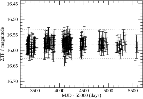
A time vs. flux plot showing a flat trend.

The light curve of WD J0234-0406 measured by the Zwicky Transient Facility. Unlike WD 1145+017, which frequently changes brightness, this white dwarf appears remarkably steady despite the high-velocity gas surrounding it. [B. Zuckerman et al. 2026]

This new star, called WD J0234-0406, shares some characteristics with the “iconic” WD 1145+017 that was first spotted mid-meal, but it also differs in an interesting way. High-resolution spectroscopy reveals that both stars have gaseous material orbiting around them along highly non-circular paths. These have been interpreted as “precessing rings of high velocity gas” that previously belonged to parent asteroids. However, while WD 1145+017 appears to flicker as bits of disintegrating asteroids pass between it and our line of sight, WD J0234-0406 is rock steady. Neither TESS nor the Zwicky Transient Facility have detected any dips in light from the star despite the evidence that solid material must have recently drizzled into the star’s atmosphere.

The researchers suggest that this relative quiet is a matter of timing. While asteroids are actively breaking up around WD 1145+017, the parent bodies that supplied the gas and dust around WD J0234-0406 may have shattered long ago and have already been either vaporized or ground down into smaller particles. All that is left over are the crumbs slowly spiraling toward the star.

Although WD J0234-0406’s meal may not be as dramatic as WD 1145+017’s feast, it’s still exciting to expand the sample of known white dwarf-asteroid interactions. And, with the upcoming release of data from the DESI survey poised to reveal the spectra of tens of thousands of white dwarfs, the sample is likely to grow again soon.

Citation

“High-velocity Circumstellar Gas Orbiting a White Dwarf Star,” B. Zuckerman et al 2026 ApJ 1004 254. doi:10.3847/1538-4357/ae23c4

The post Finishing Off an Asteroid appeared first on AAS Nova.

Diving into the Darkest Corners of the Universe with Fast Radio Bursts

5 August 2026 at 18:25

The cosmic web

Even the darkest corners of the universe are not completely empty. A recent study has used fast radio bursts to provide the first estimate of the baryon content in cosmic voids.

What’s in a Void?

Cosmological studies have revealed the large-scale filamentary structure of the universe known as the cosmic web. Chains of galaxies and galaxy clusters fall into spindly strands (or filaments) of matter overdensities, opening up cavernous cosmic voids that comprise the darkest corners of the universe. These seemingly vacant voids serve as critical test beds for cosmology, allowing researchers to constrain things like the nature of dark energy and the matter density of the universe.

Despite their name, voids are not completely empty but are instead underdensities with considerably less matter compared to the bustling filaments they border. The baryon (normal matter) content of cosmic voids has important implications for cosmological models and large-scale galactic feedback processes, but assessing how many baryons actually occupy voids has only recently become observationally accessible.

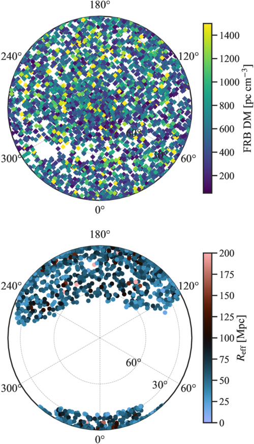
FRB and void sky maps

Sky maps centered on the north celestial pole showing the CHIME fast radio burst sample (top) and the SDSS void catalog (bottom). [Sharma et al 2026]

Fast radio bursts — brief, intense flashes of radio waves emitted by compact objects — have proven to be versatile tools for measuring both underdensities and overdensities throughout the universe. The dispersion measure of fast radio bursts, which tells us how many free electrons fall between the radio emitter and observer, can be directly used to map the baryon content along the lines of sight. Fast radio burst sight lines passing through overdensities will produce a dispersion measure excess, and those passing through underdensities will produce a dispersion measure deficit relative to the cosmic mean. Thus far, fast radio bursts have been used extensively to study overdense galaxy and cluster filaments, but their sensitivity to underdense regions like voids has yet to be explored.

Chiming In on the Baryon Search

In concept, directly stacking fast radio burst sight lines that coincide with the positions of known cosmic voids provides a direct measurement of the baryon underdensity inside voids. With no previous observational exploration of this quantity, Kritti Sharma (California Institute of Technology) and collaborators leveraged the second catalog of the Canadian Hydrogen Intensity Mapping Experiment Fast Radio Bursts (CHIME/FRB) sample in conjunction with the Sloan Digital Sky Survey (SDSS) Baryon Oscillation Spectroscopic Survey (BOSS) void catalog to provide the first observational assessment of the baryon underdensity in cosmic voids.

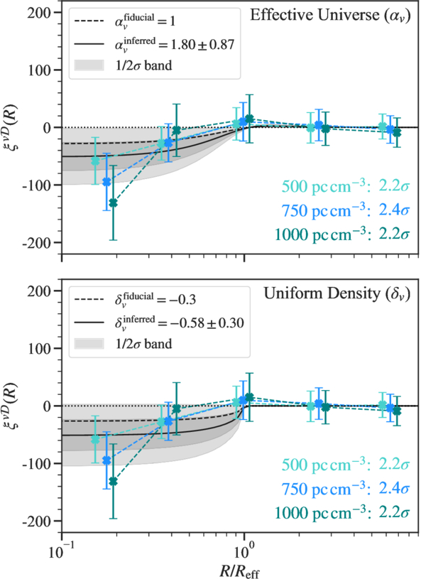
Anticorrelations between FRB dispersion measures and void positions

Anticorrelations between fast radio burst dispersion measures and void positions. There is a clear dispersion measure deficit closer to voids centers. [Sharma et al 2026]

Stacking thousands of fast radio burst sight lines that spatially align with thousands of known voids, the authors measured a statistically significant dispersion measure deficit toward void centers. This deficit indicates that, as theory predicts, baryons inhabit cosmic voids at a suppressed level. The team used cosmological models to quantify the electron density contrast between the interior and exterior of voids, finding an approximate baryon underdensity of 60% ± 30% relative to the cosmic mean. Combining this result with existing thermal scattering measurements of the cosmic microwave background, the authors estimated a mean void gas temperature of about 1.1 million kelvin — voids are occupied by a suppressed amount of warm-hot diffuse gas.

This study provides a unique approach to baryon mapping and opens up the door for future investigation of cosmic voids. While not physically containing much, voids hold vast astrophysical and cosmological significance. With the astronomical stage primed with galaxy-mapping powerhouses like the Dark Energy Spectroscopic Instrument, Vera Rubin Observatory, Nancy Grace Roman Space Telescope, and Euclid Space Telescope, cosmic voids will become a cornerstone of cosmological studies.

Citation

“Baryons in the Darkest Sites of the Universe,” Kritti Sharma et al 2026 ApJL 1006 L3. doi:10.3847/2041-8213/ae81ac

The post Diving into the Darkest Corners of the Universe with Fast Radio Bursts appeared first on AAS Nova.

EXCELlent Work, Detectives! Solving the Murder of Star Formation in Galaxies with JWST

4 August 2026 at 17:00

Arp 142

Editor’s Note: Astrobites is a graduate-student-run organization that digests astrophysical literature for undergraduate students. As part of the partnership between the AAS and astrobites, we occasionally repost astrobites content here at AAS Nova. We hope you enjoy this post from astrobites; the original can be viewed at astrobites.org.

Title: The JWST EXCELS Survey: Insights into the Nature of Quenching at Cosmic Noon
Authors: Maya Skarbinski et al.
First Author’s Institution: Johns Hopkins University
Status: Published in ApJ

How to Quench a Galaxy

Look at an image of the sky taken with a sufficiently sensitive telescope, and you’ll quickly notice that galaxies tend to cluster into two main types: blue spiral galaxies, which have flat disk shapes with a central bulge, and red elliptical galaxies, which look like spherical or elliptical balls of red stars. Blue spiral galaxies can form tens to hundreds of stars every year, while elliptical galaxies have completely stopped forming stars, meaning that some process has to transform star-forming spirals into non-star-forming, or “quiescent,” elliptical galaxies. To form the current population of massive elliptical galaxies, this process had to be common about 2–3 billion years after the Big Bang at “cosmic noon,” the period when star formation in the universe peaked. The processes that “quench” star formation in massive galaxies are still being studied, and one of the best ways to study them is to find galaxies that recently quenched and look for clues about the processes that quenched them.

Post-starburst galaxies are galaxies that have rapidly quenched after a short burst of star formation. Because these galaxies quenched so quickly and so recently, it’s often possible to find signs of whatever quenched them, like the signatures of past galaxy mergers, feedback from supermassive black hole accretion, or the shutoff of gas flowing into the galaxy. Rapid quenching is pretty uncommon now, but it was a much more common way for galaxies to quench at cosmic noon. Understanding post-starburst galaxies at cosmic noon is therefore critical for understanding the formation of massive elliptical galaxies in the local universe.

The Quest for Quenched Galaxies

Today’s article uses data from the JWST Early eXtragalactic Continuum and Emission Line Survey (EXCELS) to identify post-starburst galaxies at cosmic noon and try to determine why they quenched. EXCELS is a spectroscopic survey, so the authors get a spectrum for every galaxy. The spectrum encodes information about the galaxy’s stellar population, including the mass of stars in the galaxy, the number of stars forming every year, and the history of star formation throughout the galaxy’s life.

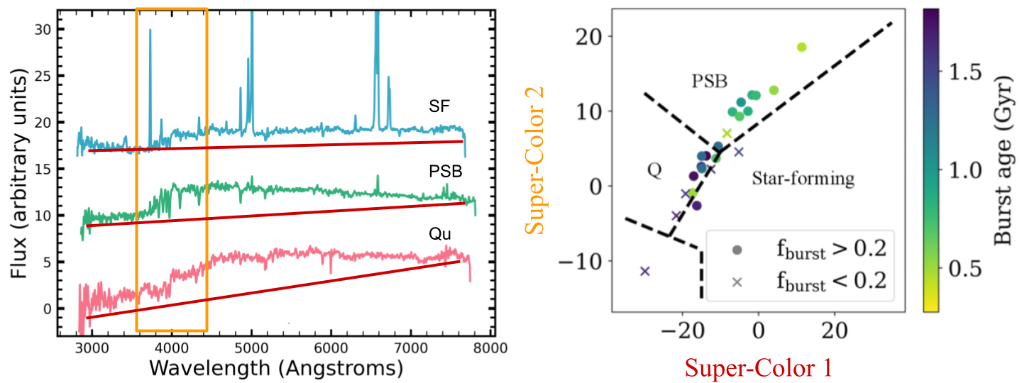
The authors use a technique called principal component analysis to further divide the sample into young and old post-starbursts. Principal component analysis is a machine-learning technique that learns the most important features of a data set. This technique is used for “dimension reduction,” or reducing the number of data points needed to learn something about the object. A typical spectrum has hundreds or even thousands of data points, which means performing data analysis on a spectrum can be very computationally expensive. Principal component analysis takes these thousands of data points and learns broad patterns that correlate with each other. These patterns are called “supercolors” in the context of spectral data, and they encode things like the overall shape and color of the spectrum as well as the spectral shape around key features (see Figure 1 for a visualization). Since the overall shape, color, and emission/absorption line features of a spectrum come from the galaxy’s stellar population, this method can be used to identify galaxies with lots of star formation a billion years ago but very little star formation today — in other words, post-starburst galaxies.

demonstration of principal component analysis for spectra of different types of galaxies

Figure 1: An example of principal component analysis for sample star-forming (SF), quiescent (Qu), and post-starburst (PSB) galaxy spectra (left-hand side). Principal component analysis simplifies a many-dimensional data set (for example, spectra) into fewer dimensions. In this case, Super-Color 1 measures the overall color of the spectrum (shown on the left-hand side as the slope of the spectra, marked with red lines), while Super-Color 2 measures the shape of the spectrum around 4,000 angstroms (orange box). The authors use principal component analysis to identify post-starburst galaxies for further analysis (right-hand side). [Adapted from Skarbinski et al. 2026]

The authors apply principal component analysis to the galaxies in their sample and find that 11 of the galaxies in their sample are classified as post-starburst, 9 are quiescent, and 4 still have some star formation. To further analyze the stellar populations of the post-starbursts in their sample, the authors use a program called Bagpipes to fit the galaxies’ spectra. Bagpipes is a spectral energy distribution fitting software, which means that it takes the observed spectrum of a real galaxy and tries to match it to a library of different stellar spectra. By measuring the relative contribution of different kinds of stars (which all have different lifetimes), Bagpipes can compute the likely history of star formation in the galaxy (e.g., when the star formation rate peaked) as well as the present-day properties of the galaxy (things like the mass in stars versus dust and the current star formation rate). The authors use the galaxies’ star formation histories to try to find clues as to how they quenched.

How Quickly Do Post-Starbursts Quench?

First, the authors measure something called a “quenching timescale,” which they define as the length of time between when the galaxy’s star formation rate peaked and when it fell low enough that the galaxy was quenched. The quenching timescale depends on which process shut down star formation in the galaxy — feedback from black hole accretion or star formation should cause fast quenching, while galaxies that are starved of gas from the intergalactic medium should quench more slowly. The authors find that 15 of their galaxies quenched in under 500 million years, 6 took between 500 million and 1 billion years, and 3 took longer than 1 billion years to quench. The galaxies that had the highest peak star formation rates quenched the fastest, suggesting that feedback from star formation could have played a role in quenching these galaxies.

plots showing possible evolutionary tracks for two example galaxies

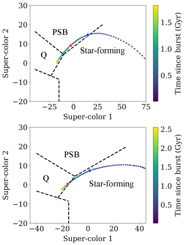
Figure 2: Possible evolutionary tracks in supercolor for two example galaxies as they quench. The galaxy in the top panel quenches quickly and has post-starburst supercolors for about a billion years, while the galaxy in the bottom panel quenches without ever going through the post-starburst phase. The authors use these tracks to determine how important the post-starburst phase is for quenching massive galaxies. [Skarbinski et al. 2026]

Next, the authors measure how important the post-starburst phase is to form massive quiescent galaxies. Not all galaxies that quench go through a post-starburst phase; some objects, especially those that quench slowly, will transition directly from star forming to quiescent. The authors use the star formation histories from their spectral energy distribution fits to predict how the galaxies’ supercolors changed after their star formation peaked (Figure 2) and find that six of the nine quiescent galaxies went through a post-starburst phase in the past, while the other three did not. For the objects that went through a post-starburst phase, the median time spent as a post-starburst was around 600 million years.The authors can use this measured “visibility timescale” to constrain whether the post-starburst phase is important for forming massive quiescent galaxies. If the fraction of post-starburst galaxies in a sample is high, that can be for two reasons: either a larger fraction of galaxies will eventually go through a post-starburst phase, or the post-starburst phase is very long, making it easy to find post-starburst galaxies. Using the measured timescale of 600 million years and combining with results from another article, the authors find that 40% of quiescent galaxies likely went through a post-starburst phase; for the more massive end of the sample, this fraction increases to around 73% due to the shorter visibility timescale. This suggests that the post-starburst phase is very important for forming the kind of massive quiescent galaxies we see in the local universe.

While the post-starburst phase is important, the different quenching timescales present across the sample suggest that multiple pathways existed to quench galaxies at cosmic noon, similar to what has been found in less-distant galaxies and at cosmic noon in other samples. This is also supported by the fact that four of the five galaxies with sufficient data show evidence of an actively accreting supermassive black hole that may help shut down star formation in many (but perhaps not all) massive galaxies. While the precise processes that quench massive galaxies are still uncertain, one thing is clear: JWST EXCELS at solving the mystery!

Original astrobite edited by Anavi Uppal.

About the author, Margaret Verrico:

I am a fourth-year graduate student at the University of Illinois Urbana-Champaign. I study the connection between supermassive black hole transients and their host galaxies. I am also an avid knitter and reader, and I am passionate about opening up STEM opportunities for people of all backgrounds.

The post EXCELlent Work, Detectives! Solving the Murder of Star Formation in Galaxies with JWST appeared first on AAS Nova.

Featured Image: Citizen Science and Solar Structure

3 August 2026 at 17:00

solar corona during a solar eclipse

During the 8 April 2024 solar eclipse, the path of totality swept across North America, dazzling millions of skygazers. Scattered along this path were 82 viewing sites of the Dynamic Eclipse Broadcast Initiative citizen science project, which aimed to observe the dynamics of the tenuous solar corona. Though poor weather dashed many observers’ hopes, the project managed to collect data at 11 sites spanning 2,700 kilometers, capturing 49 minutes of coronal behavior. The image above shows the solar corona as seen during totality from one of the DEB Initiative sites. In a recent research article, Matthew J. Penn (Southern Illinois University Carbondale; Tucson Amateur Astronomy Association) and collaborators described the results of the Initiative’s viewing efforts, including identification of downflows and outflows, plumes, coronal loops, and apparent motion of background stars. To learn more about these observations of the solar corona, be sure to check out the full article linked below.

Citation

“Structure and Dynamics of the Inner Corona Measured from the DEB Initiative 2024 Eclipse Image Sequence,” Matthew J Penn et al 2026 ApJL 1006 L25. doi:10.3847/2041-8213/ae8797

The post Featured Image: Citizen Science and Solar Structure appeared first on AAS Nova.

Spying on a Split Comet

31 July 2026 at 17:00

240P

Traversing through the solar system, a comet split in two, and a recent study used six months of observations to investigate when and why.

A Split Comet

Orbit map

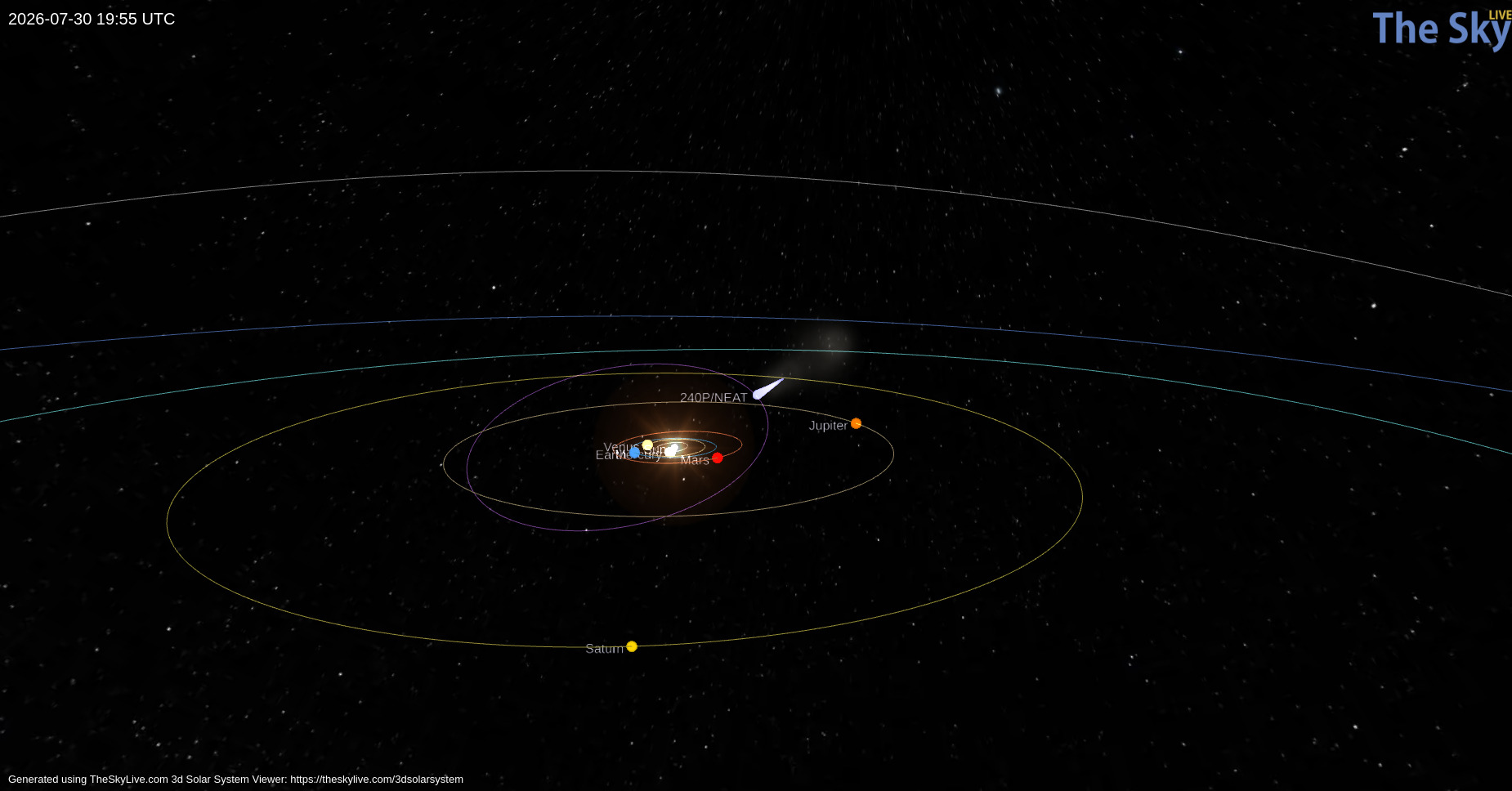
Orbital path of 240P/NEAT (purple) and the position of the comet on 30 July 2026 (light blue teardrop). Click to enlarge. [TheSkyLive]

While we often think of comets as icy remnants of the solar system’s formation that populate the Kuiper Belt and Oort Cloud, some comets make their homes closer to the Sun. One such class, known as Jupiter-family comets, traveled from the Kuiper Belt to short orbital periods (less than 20 years) whose paths through the solar system are shaped by Jupiter’s gravity. Discovered in 2002, 240P/NEAT is a Jupiter-family comet that loops between Jupiter and Mars on a 7.6-year orbit. Making close approaches to Jupiter, 240P experiences frequent, strong interactions with the gas giant that can alter the comet’s orbit and cause sudden bursts in brightness as ice and dust are heated and outgassed from the comet’s surface.

Most recently, 240P swept closest to Jupiter in July 2007, shifting the comet’s perihelion distance (closest approach to the Sun) from 2.5 to 2.1 au, and several long-lived bursts in brightness in 2018/2019 could have been spurred by this orbital shift. Excitingly, a fainter comoving object, 240P-B, was first reported in June 2025 as the comet headed toward perihelion — at some point recently, 240P had split in two!

Over the last century, numerous split comets have been recorded, but detailed physical studies of these objects are rare. With growing evidence suggesting splitting and disintegration are the primary mechanisms of comet destruction, understanding the properties and cause of 240P’s split is imperative.

Observing 240P

With 240P on the move to perihelion, David Jewitt (University of California, Los Angeles) and collaborators monitored the comet from October 2025 to April 2026 to establish the likely cause of its split. Employing the Alhambra Faint Object Spectrograph and Camera on the 2.56-meter Nordic Optical Telescope, the authors obtained detailed imaging of the comet from two months before to four months after perihelion to characterize both components.

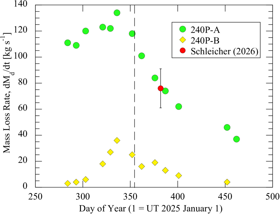
Tracking both photometric and morphological changes across their observations, the authors estimated the dust-loss rates, physical sizes, and separation speed of 240P-A and 240P-B. The brighter component, 240P-A, has an estimated radius between 400 and 600 meters and a dust-loss rate almost four times higher than 240P-B. Because 240P-B is fainter, its radius is harder to constrain observationally. From its lower dust-loss rate and lower brightness, the authors estimated a radius around 300 meters (and no smaller than 50). Based on how the separation of the two comet pieces changes over time, the authors determined that the split of 240P occurred at least three years before their observations.

dust mass-loss

Dust mass-loss rates for 240P-A (green circles) and 240P-B (yellow diamonds) over the course of the observations. Both components peak shortly before perihelion (dashed vertical line). Click to enlarge. [Jewitt et al 2026]

Source of the Split

How exactly did this fragmented comet get this way? The authors considered a number of comet-splitting mechanisms: tidal forces, asteroid impact, pressure buildup below the comet’s surface, thermal stresses, and rotational instability. Given the comet’s orbit, it has not had close enough encounters with the Sun or other planets for tidal forces to be the culprit, and it traverses well above the asteroid belt, avoiding collisions. Pressure buildup and thermal stresses can fracture comets, but both are unlikely to launch such a large fragment as seen in this system.

This leaves rotational instability as the likely source of 240P’s split. Outgassing torques lead to rotational instability, especially in subkilometer comets like 240P, and 240P has exhibited recent outgassing. In addition, the separation speed between the 240P components is comparable to the escape speed of the primary comet, which is expected for rotational breakup. To confirm this hypothesis, future observations measuring the rotation period of 240P are necessary, but this study adds to the small number of split-comet observations that aid in understanding comet destruction.

Citation

“Investigation of Split Comet 240P/NEAT,” David Jewitt et al AJ 172 113. doi:10.3847/1538-3881/ae83ac

The post Spying on a Split Comet appeared first on AAS Nova.

Monthly Roundup: The Fourth Catalog of Gravitational Wave Events from LIGO, Virgo, and KAGRA

29 July 2026 at 17:00

Illustration of gravitational waves emanating from a pair of black holes approaching a merger

A recent Focus Issue of the Astrophysical Journal Letters describes the fourth version of the catalog of gravitational wave events (GWTC-4.0) from the Laser Interferometer Gravitational Wave Observatory (LIGO), the Virgo interferometer, and the Kamioka Gravitational Wave Detector (KAGRA).

This catalog contains transient gravitational wave events recorded through January 2024, during the observatories’ fourth observing run, which concluded in November 2025. GWTC-4.0 displays the results of significant improvements to our suite of gravitational wave detectors, including higher-powered lasers and reduced quantum noise. A fifth catalog of gravitational wave events was released in Spring 2026, with the accompanying scientific articles being submitted to the Astrophysical Journal and the Astrophysical Journal Letters.

This Monthly Roundup consists of short descriptions of each of the currently published research articles in the LIGO–Virgo–KAGRA Gravitational Wave Transient Catalog (GWTC): Release 4 Focus Issue. Each snippet links to the corresponding research article, and the Focus Issue landing page is linked at the bottom of this post. Be sure to revisit the landing page to catch new articles as they’re published!

Introducing GWTC-4.0

timeline of gravitational wave observatories' observing runs

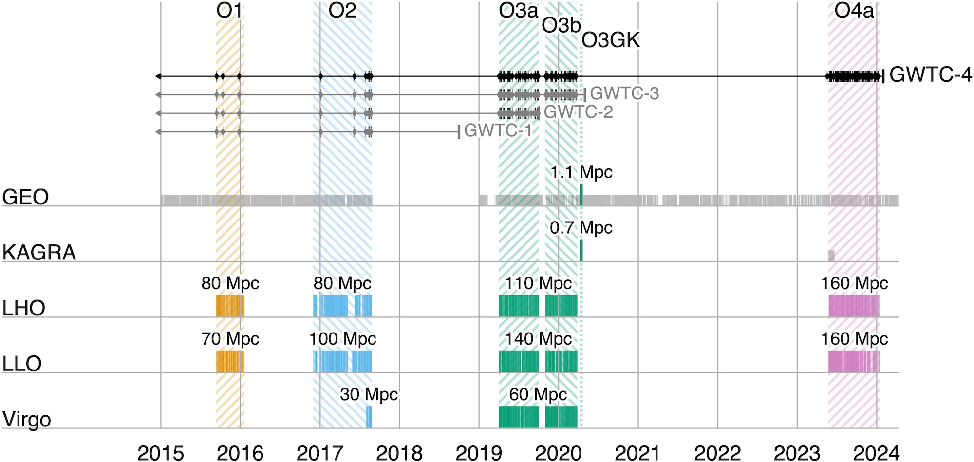
A timeline showing observing runs between 2015 and 2024. Click to enlarge. [LVK Collaboration 2025]

First up, the collaboration orients the reader to many important aspects of the catalog and the articles contained in the Focus Issue. This article describes how four detectors, each with two arms 3–4 kilometers long, monitor gravitational waves from Hanford, Washington; Livingston, Louisiana; Santo Stefano a Macerata, Italy; and Hida, Japan. These detectors work in concert, ready to receive signals from the universe during coordinated observing runs separated by periods of downtime for construction and commissioning. During these pauses, a smaller instrument, the German–British GEO600 gravitational wave detector, has kept an ear out for signals and will continue to do so until the end of 2026.

After these detectors record subtle spacetime squiggles from compact objects colliding millions to billions of light-years away, the collaboration converts the raw signals into the data contained in catalogs like GWTC-4.0. This process involves modeling the gravitational wave signals, filtering them to identify candidate transients, and pinpointing the most significant events.

After collecting and cleaning the signals, the collaboration undertakes a critical step: making their data accessible to researchers and the public. The data are available through the Gravitational Wave Open Science Center, and the Focus Issue article on open data describes how to navigate the online portal, how the datasets archived online are structured, and how the data were calibrated.

Science Results

This fourth version of the gravitational wave transient catalog greatly expands the sample of gravitational wave transients recorded by detectors across the globe. Including events from previous catalogs, GWTC-4.0 brings us to 218 events for which the probability of the source being astrophysical in nature is more than 50% and for which there is little chance of the signal being an instrumental artifact. This represents a more than 100% increase in the number of recorded gravitational wave events fulfilling this criterion, broadening our understanding of colliding compact object pairs. This release also includes some superlative signals, such as the most massive black hole binary with a low false-alarm rate and the highest signal-to-noise ratio for a gravitational wave event thus far.

Detected in November 2023 by both LIGO Hanford and LIGO Livingston, GW231123 is in many ways an exceptional gravitational wave transient. The total mass of the merging components appears to be between 190 and 265 solar masses, and the false-alarm rate for this signal is less than one per year. This makes it the most massive merger event with such a low false-alarm probability. The two components also appear to have high spins, which complicates the interpretation of the signal with existing models. A binary black hole merger in which one or more components lies within the pair-instability mass gap is the likeliest explanation for this signal, but the authors also present alternative scenarios, such as a core-collapse supernova or a gravitationally lensed gravitational wave signal.

GW230814 gravitational wave signal

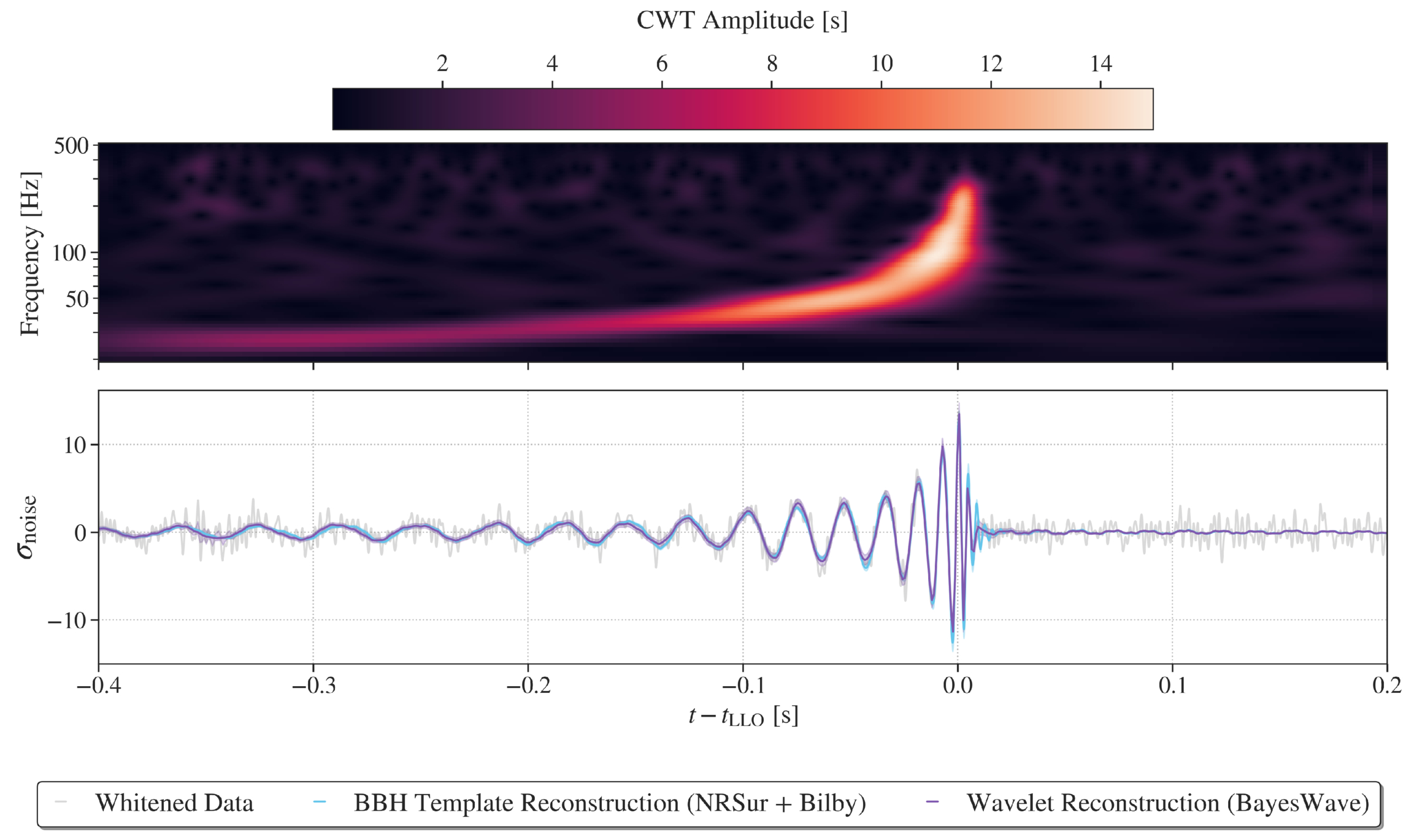
Representations of the GW230814 gravitational wave signal. Click to enlarge. [LVK Collaboration 2026]

GW230814, which was detected only by LIGO Livingston, is the loudest signal in the catalog. This signal is consistent with the collision of two black holes, each of roughly 30 solar masses. During the analysis of this signal, the team discovered potential deviations from the predictions of general relativity in the ringdown phase, when the remnant black hole settles into its final shape. Without a detection from another facility to corroborate this finding, it’s difficult to pinpoint the cause of the deviation, but the team could not rule out statistical noise fluctuations as the source.
Plot of the differential merger rate

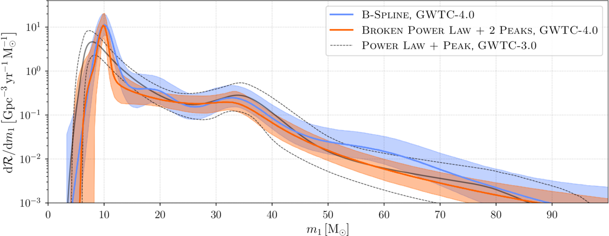
Plot of the differential merger rate as a function of the mass of the more massive of the two merger components. This shows overdensities at 10, 35, and possibly 20 solar masses. Click to enlarge. [LVK Collaboration 2026]

Surveying merging black holes and neutron stars on the population level, the team analyzed 158 gravitational wave signals from the current catalog. This analysis supported findings from previous transient catalogs, including multiple overdensities in the distribution of merging black hole masses, broadly distributed neutron star masses, and an increase in the merger rate with redshift. The new data strengthened certain previously identified trends, such as an increase in the width of the effective spin distribution with redshift, and weakened others.

The full list of articles in the GWTC-4.0 Focus Issue can be found here.

Citation

“GWTC-4.0: An Introduction to Version 4.0 of the Gravitational-Wave Transient Catalog,” A. G. Abac et al 2025 ApJL 995 L18. doi:10.3847/2041-8213/ae0c06

“GWTC-4.0: Methods for Identifying and Characterizing Gravitational-Wave Transients,” A. G. Abac et al 2026 ApJL 1004 L21. doi:10.3847/2041-8213/ae447b

“Open Data from LIGO, Virgo, and KAGRA Through the First Part of the Fourth Observing Run,” A. G. Abac et al 2026 ApJ 1004 232. doi:10.3847/1538-4357/ae211e

“GWTC-4.0: Updating the Gravitational-Wave Transient Catalog with Observations from the First Part of the Fourth LIGO–Virgo–KAGRA Observing Run,” A. G. Abac et al 2026 ApJL 1004 L22. doi:10.3847/2041-8213/ae2c74

“GW231123: A Binary Black Hole Merger with Total Mass 190–265 M⊙,” A. G. Abac et al 2025 ApJL993 L25. doi:10.3847/2041-8213/ae0c9c

“GW230814: Investigation of a Loud Gravitational-Wave Signal Observed with a Single Detector,” A. G. Abac et al 2026 ApJL 1004 L23. doi:10.3847/2041-8213/ae2ad3

“GWTC-4.0: Population Properties of Merging Compact Binaries,” A. G. Abac et al 2026 ApJL 1005 L51. doi:10.3847/2041-8213/ae771e

The post Monthly Roundup: The Fourth Catalog of Gravitational Wave Events from LIGO, Virgo, and KAGRA appeared first on AAS Nova.

The “Rhythm” of the Interstellar Medium

28 July 2026 at 17:00

Messier 17

Editor’s Note: Astrobites is a graduate-student-run organization that digests astrophysical literature for undergraduate students. As part of the partnership between the AAS and astrobites, we occasionally repost astrobites content here at AAS Nova. We hope you enjoy this post from astrobites; the original can be viewed at astrobites.org.

Title: The Rhythm of the ISM: Tracing the Timescales of Gas Evolution and Star Formation Across Galactic Environments
Authors: Zuzanna Kocjan and Vadim A. Semenov
First Author’s Institution: University of Maryland
Status: Published in ApJ

The Connection Between Gas and Star Formation in Galaxies

Stars are born in the interstellar medium (ISM) when cold, dense clouds of gas become unstable and collapse under gravity. Despite their plentiful reservoirs of gas, galaxies convert only a small fraction of this material into stars, making star formation a surprisingly inefficient process. A key factor behind this inefficiency is stellar feedback: radiation, stellar winds, and supernova explosions from young stars can inject energy and momentum into the surrounding gas, heating, stirring, and dispersing it. In this way, stellar feedback shapes future star formation across scales ranging from individual regions in the ISM to whole galaxies.

An important tool astronomers use to study star formation is the Kennicutt–Schmidt relation, which links the amount of gas in a galaxy to the rate at which stars form. More specifically, it relates the gas surface density, Σgas, to the star formation rate surface density, ΣSFR. (For more on this relation, see this Astrobites article on a classic research article.) However, this law is underpinned by a crucial ingredient: timescales. In particular, the pace of star formation depends both on how quickly galactic gas is cycled into star-forming material and on how rapidly those regions convert gas into stars once they form. Today’s article investigates the physical origin of star-formation scaling relations behind the Kennicutt–Schmidt law by building on a simple theoretical framework for the ISM.
Consider a Kettle of Boiling Water…

In a given region of a galaxy, the ISM consists of gas in either an actively star-forming state or an inert, non-star-forming state, depending on whether it is dense and unstable enough to collapse (as illustrated in Figure 1). The transition of non-star-forming gas into the star-forming state occurs on the supply timescale, τ+. Conversely, the dispersal of star-forming gas back into a non-star-forming state is characterized by the removal timescale, τ–. As a helpful analogy, the authors compare this process to water boiling in a kettle: the ISM is continuously “boiling,” with gas moving between active and inactive states. Meanwhile, the total gas reservoir gradually decreases, analogous to water slowly evaporating as the kettle boils. The gas depletion time, τ*, therefore represents the timescale over which the available gas would be exhausted by star formation.
Schematic of the gas cycling framework

Figure 1: Schematic of the gas cycling framework used in the authors’ theoretical model for how gas is converted into stars, which takes into account a supply, removal, and depletion timescale. [Adapted from Kocjan and Semenov 2026]

Building on this picture of gas cycling, the authors turn to simulated galaxies, where the motion and evolution of the gas can be followed directly. By tracking how gas flows through the ISM in the simulations, they derive the three characteristic timescales above — τ+, τ–, and τ* — that describe how gas is supplied to, removed from, and ultimately consumed by star formation. The goal is to connect the small-scale physics of the ISM to the large-scale star formation efficiencies and scaling relations observed across galaxies.

The Timescales of the Interstellar Medium

To explore how gas and star formation are connected across different galactic environments, the authors analyze three simulated systems: a dwarf galaxy, a Milky Way–like galaxy, and a gas-rich starburst galaxy, as shown in Figure 2. Despite spanning very different physical regimes, the galaxies exhibit remarkably similar trends in the fraction of gas actively forming stars as a function of Σgas​. This suggests that the amount of star-forming gas is governed primarily by local interstellar conditions, since regions with higher gas surface densities tend to contain denser, more strongly self-gravitating gas.

galaxy simulations and star-forming gas fraction

Figure 2: Using simulations (left to right) of an isolated intermediate-mass dwarf galaxy, Milky Way–like galaxy, and gas-rich galaxy, the authors measure the star-forming gas fraction versus the gas surface density (right). [Adapted from Kocjan and Semenov 2026]

To further understand this trend, this study then applies the authors’ theoretical framework to determine the timescales of ISM gas cycling on the scales of individual star-forming regions. These include the timescales for the formation, dispersal, and local depletion of star-forming gas as described above: τ+, τ−, and τ∗, which also exhibit strong correlations with the gas surface density (see Figure 3). Specifically, the timescale for supplying gas into the star-forming state is linked to the rate at which turbulence redistributes material through the galactic disk. The depletion timescale, over which star-forming gas is turned into stars, decreases at higher Σgas​, since denser regions more efficiently collapse and form stars. By contrast, the removal timescale is comparatively short, reflecting how quickly feedback and changes in local equilibrium can disrupt star-forming clouds. In this way, the “boiling kettle” framework is able to capture the major processes driving small-scale gas evolution.
Scaling relations between the supply, depletion, and removal times

Figure 3: Scaling relations between the supply (left), depletion (middle), and removal (right) times in kiloparsec-scale regions of the simulated galaxies (shown in different colors). Based on the measurements from the simulations, the authors introduce a parameterized model for the gas cycling framework, as defined in the equations. [Adapted from Kocjan and Semenov 2026]

The cycling of gas through different phases of the ISM offers a useful framework for understanding how galaxies form stars. In the relatively well-ordered systems studied here, this balance can be described in simple terms; however, it is likely to become more complex in extreme environments where additional physical processes — such as those operating in the early stages of galaxy formation — play a significant role. Even so, these results highlight how key galactic properties can emerge naturally from the interplay between galaxy-scale dynamics, ISM turbulence, and the state of star-forming gas.

Original astrobite edited by Jayde Willingham.

About the author, Shalini Kurinchi-Vendhan:

After studying astrophysics and literature at Caltech, I moved onto a Fulbright Fellowship in Heidelberg, Germany. I’m passionate about using computer simulations to explore supermassive black holes and galaxy evolution — but I also love poetry and traveling.

The post The “Rhythm” of the Interstellar Medium appeared first on AAS Nova.

First-Generation Stars Provide Better Fit than a Black Hole for Early-Universe Gas Clump

27 July 2026 at 17:00

Star formation in the early universe.

An unusual clump of gas 450 million years after the Big Bang may contain stars hailing from the universe’s elusive first generation of stars. New research examines an alternative explanation involving an accreting black hole.

Meet Hebe

Hebe and GN-z11

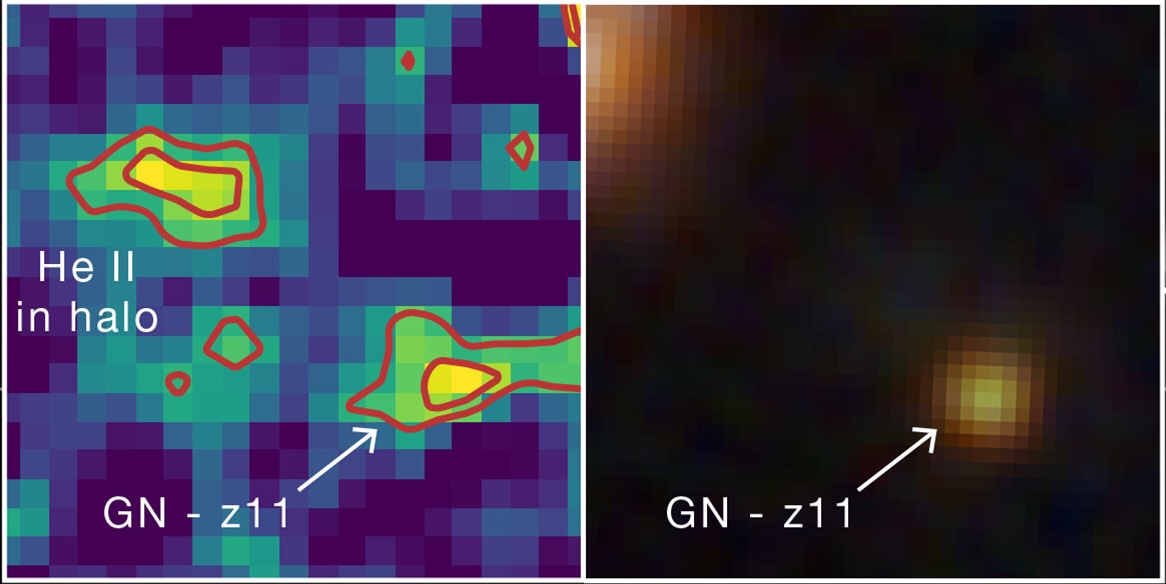
Hebe is visible in the image on the left as a prominent blob of helium emission up and to the left from GN-z11, a luminous galaxy hosting an accreting supermassive black hole. On the right is an infrared image of the same region, in which Hebe is not visible. Click to enlarge. [Adapted from NASA, ESA, CSA, Ralf Crawford (STScI)]

Initially spotted in 2024, an early-universe gas clump nicknamed Hebe has now been identified as a possible hiding place of Population III (Pop III) stars — the universe’s first generation of stars. Pop III stars are thought to be massive and chemically pristine, containing only hydrogen, helium, and a whisper of lithium. This exciting hypothesis was prompted by the detection of recombination lines from helium, which could be ionized by the high-energy radiation of the first stars.

Before the community settles on this exciting explanation, however, the hypothesis must withstand all the tests astronomers can throw at it. In a recent research article, Junehyoung Jeon, Tae Bong Jeong, and Saiyang Zhang (The University of Texas at Austin) along with Volker Bromm (The University of Texas at Austin) attempted to explain Hebe’s properties in another way.

Considering Alternatives

Hebe glows with distinctive helium emission that requires a source of high-energy radiation. This radiation could be provided by a cluster of Pop III stars, but it could also, in theory, arise from an accreting supermassive black hole embedded within the gas clump.

predicted Pop III star mass in Hebe

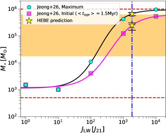
Predicted total mass of Hebe’s Pop III stars as a function of the Lyman–Werner flux from the nearby galaxy GN-z11. Click to enlarge. [Jeon et al. 2026]

The authors used models to explore both possibilities. For the first scenario, in which the telltale helium emission is driven by a cluster of Pop III stars, the team calculated the maximum possible mass of the cluster, which sets how much high-energy radiation is produced. The cluster mass is moderated by high-energy radiation from another source: GN-z11, a starburst galaxy situated about 10,000 light-years from Hebe. For the second scenario, the team modeled the spectral energy distribution arising from a supermassive black hole — either a direct-collapse black hole or a primordial black hole — accreting pristine gas from the surrounding cloud.

Still a Leading Explanation

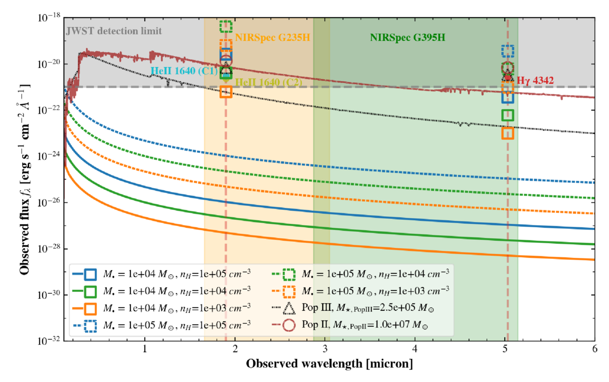
While the black hole scenario could, with reasonable black hole masses, gas densities, and accretion rates, reproduce individual flux measurements drawn from JWST observations, this hypothesis struggled to simultaneously match multiple measurements. The Pop III star cluster scenario, with a cluster mass of a few hundred thousand solar masses, provided the best fit to the JWST data.

modeled spectral energy distributions for Hebe based on the black hole or Pop III star hypotheses

Modeled spectral energy distributions (lines) and predicted line flux densities (open symbols) for the accreting black hole, Pop III star, and Pop II (second-generation) star hypotheses. The observed JWST line fluxes are shown as filled circles. Click to enlarge. [Jeon et al. 2026]

As a final test, the team introduced a third possibility involving a population of second-generation stars, which are more chemically enriched than Pop III stars. While this model fit well, the number of stars necessary to match the data — roughly 10 million — would produce a stellar continuum detectable (but so far not seen) by JWST.

While a cluster of Pop III stars is still the leading explanation for Hebe’s properties, the team noted that the Pop III star and black hole hypotheses aren’t mutually exclusive; Hebe could very well harbor a primordial black hole and a smattering of Pop III stars. Regardless of what powers its characteristic helium emission, Hebe offers an enticing glimpse into the early universe, and more work is needed to understand this intriguing object.

Citation

“What Is Powering the Enigmatic He II Emitter Hebe: The First Stars or Black Holes?” Junehyoung Jeon et al 2026 ApJ 1006 27. doi:10.3847/1538-4357/ae7bea

The post First-Generation Stars Provide Better Fit than a Black Hole for Early-Universe Gas Clump appeared first on AAS Nova.

Noble Gases Along for the Ride

24 July 2026 at 17:00

A rendering of an orange and grey planet against a dark background.

What can some neon trapped in a chunk of rock tell us about Earth’s formation and the protosolar nebula? Quite a lot, as detailed in a recent study in The Planetary Science Journal.

Noble Mysteries

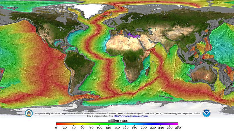
By analyzing rocks pulled from mid-ocean ridges, geologists have concluded that there are tiny amounts of noble gases in the deep interior of Earth. That’s a strange statement upon reflection: how did these gases, which are famously apathetic to essentially all other elements, end up embedded within rocks thousands of kilometers underground? Since their passivity rules out the potential of a chemical reaction that formed them in place, they must have been in the mantle since the very beginning of Earth’s history.

A map of Earth with the continents shown normally but the sea colored according to age.

A map illustrating the age of the seafloor. Mid-ocean ridges stand out clearly in red. By sampling material from these ridges, planetary scientists can infer the composition of Earth’s deep interior. Click to enlarge. [Mr. Elliot Lim, CIRES and NOAA/NCEI]

There are a few scenarios for how this could have happened. Though it’s possible that these inert species were delivered to the early Earth encapsulated within primitive meteorites or in solids contaminated by ions from the solar wind, at least some fraction of these elements likely came directly from the gaseous nebula that surrounded the earliest protoplanets.

That last option is especially exciting to present-day planetary scientists interested in constraining Earth’s formation history because it requires some very specific conditions. Since light noble gases like neon don’t dissolve well in seawater, they must have dissolved into a magma ocean — meaning the nebula was still around when Earth was large enough to have a molten surface. That already restricts us to a very specific time in the solar system’s history, but it doesn’t say much about the specific size of the proto-Earth other than “big,” and it doesn’t say much about the state of the nebula other than “it existed.” Recently, Vincent Savignac and Eve Lee (University of California, San Diego; McGill University) successfully refined these constraints to pin down information about both the early Earth and the nebula that surrounded it.

Infant Earths

Savignac and Lee began by growing a grid of infant Earths on their computers via models of gas accretion and atmosphere–magma interactions. Each simulation started with a different proto-Earth mass and nebular density, and each one yielded a different amount of neon in Earth’s deep interior. Excitingly, only a small handful of the scenarios tested ended up with values similar to those observed.

A cartoon of small cores surrounded by gaseous envelopes eventually merging into the Earth.

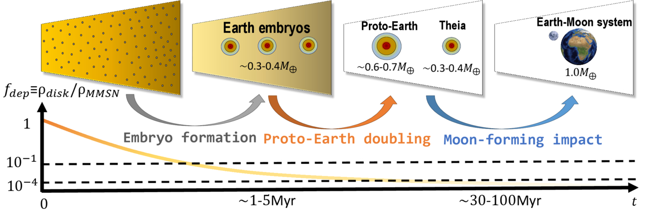
A schematic of Earth’s formation via embryo formation (when the noble gases enter the mantle) followed by mergers. Click to enlarge. [Savignac & Lee 2026]

On the mass axis, the team found a narrow range of acceptable conditions. If a proto-Earth was less than about 20% of Earth’s present-day mass, it couldn’t accrete much gas. This let it cool rapidly, freezing the magma ocean and shutting down neon dissolution before too much could be trapped inside. On the other hand, if a proto-Earth was more than about 40% of Earth’s present-day mass, it would accrete too much gas, stay molten for too long, and be left with too much neon. On the density axis, the researchers found that when the nebula accreted on to the proto-Earth, it must have been fairly depleted compared to its initial density. This implies that the whole process happened at the end of the nebula’s life, just before it was completely blown away by the proto-Sun.

Savignac and Lee demonstrated that these constraints are robust against the later stages of Earth’s evolution. In its later years, Earth either suffered or benefited from a giant impact, depending on your feelings about the Moon, but the researchers showed that this event doesn’t pose a problem for their models. Overall, this study builds a delightful link between rocks from our deep oceans and the particulars of Earth’s formation, demonstrating the unique power of planetary science to tie together different scientific fields.

Citation

“Constructing the Earth’s Formation History Using Deep Mantle Noble Gas Reservoirs,” Vincent Savignac and Eve J. Lee 2026 Planet Sci. J. 7 135. doi:10.3847/PSJ/ae64f7

The post Noble Gases Along for the Ride appeared first on AAS Nova.

Researchers Spot Hydrocarbons Surprisingly Close to a Quasar Pair

22 July 2026 at 17:00

J0749+2255

Researchers have detected molecules containing rings and chains of carbon atoms in the vicinity of a rare pair of quasars. The trends in the distribution of these molecules are unexpected, suggesting that more work is needed to understand the conditions surrounding active supermassive black holes.

Infrared Eyes on Molecules in Space

skeletal formulae of aromatic and aliphatic molecules

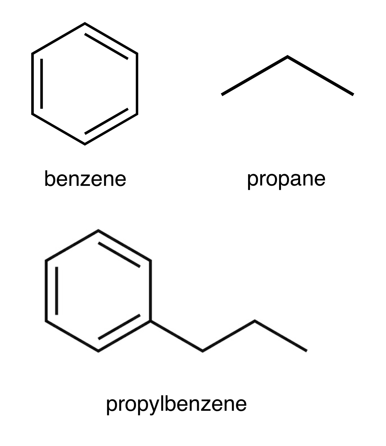
Examples of aromatic and aliphatic hydrocarbons. Benzene (top left) is the simplest aromatic molecule. Propane (top right) is a simple aliphatic molecule. Propylbenzene (bottom) is an aromatic molecule with an aliphatic chain branching off of it. In these “skeletal” formulae, there is a carbon atom at each vertex, and the remaining atoms (not depicted) are all hydrogens. Single lines indicate single chemical bonds, and double lines indicate double bonds. [Wikipedia; Public Domain]

Across the universe, atoms are combining to form molecules, and our ability to study molecules in distant realms has never been better. JWST is particularly attuned to emissions from molecules engaged in a kind of chemical yoga, stretching their bonds and flexing the angles between their atoms.

JWST’s sensitive infrared eyes have allowed researchers to study the distribution, creation, and destruction of both aromatic (containing one or more rings of carbon atoms in which certain electrons spread out within the ring) and aliphatic (containing chains of carbon atoms) hydrocarbons. These molecules have been spotted in a wide array of environments, and now, astronomers are finding them in more distant and more extreme environments than ever before.

Distant Discovery

SDSS J074922.96+225511.7, or J0749+2255 for short, is a quasar pair seen 3 billion years after the Big Bang. The two feasting supermassive black holes are roughly 12,000 light-years apart, giving researchers a glimpse into the late stages of a galaxy merger and a harsh environment in which to study the survival and destruction of molecules.

Researchers studying J0749+2255 with JWST have previously reported the detection of a 3.3-μm emission feature from aromatic molecules. Now, C. E. Mentzer (University of Missouri), Aigen Li (University of Missouri), and Xuejuan Yang (Xiangtan University) have analyzed JWST spectra of J0749+2255 and found not just widespread aromatic emission at a rest-frame wavelength of 3.3 μm, but also aliphatic emission at 3.4 μm, which they attribute to carbon chains branching off from the aromatic molecules. This likely makes J0749+2255 the most distant galaxy in which both aromatic and aliphatic emission has been detected.

analysis results showing the aliphatic fraction across the quasars and the surrounding region

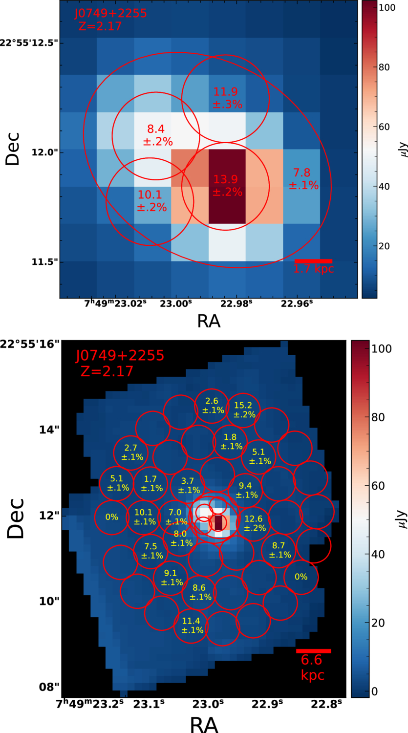
Aliphatic fractions in the bright central region surrounding the two quasars (top) and in the outer regions (bottom). [Mentzer et al. 2026]

Unexpected Trends

Mentzer, Li, and Yang subdivided the observations into 47 regions and measured the strength of the 3.3- and 3.4-μm features in each region. This analysis found strong aromatic emission nearest the quasars and showed that the fraction of carbon atoms bound up in aliphatic chains is highest close to the quasars.

Both of these findings are unexpected: the harsh radiation environment near the two active black holes is thought to break apart chains of carbon atoms attached to aromatic rings (which should decrease the 3.4-μm emission) and possibly destroy small aromatic molecules (which should decrease the 3.3-μm emission) — yet both of these features are strongest near the quasar cores where the radiation should be most capable of molecular destruction.

The authors speculated that the analysis regions centered on the quasars are large enough that they contain gas that hasn’t been pummeled by the quasars’ intense radiation and outflows, leaving molecules intact and able to produce the observed emission. However, this doesn’t explain the trend of stronger 3.3- and 3.4-μm emission closer to the quasars — necessitating further research into the emitting behavior of aromatic and aliphatic molecules under the extreme conditions of a dual quasar’s neighborhood.

Citation

“Widespread Detection of Aromatic and Aliphatic Emission in the Dual Quasar J0749+2255 at Cosmic Noon,” C. E. Mentzer et al 2026 ApJL 1005 L38. doi:10.3847/2041-8213/ae7e86

The post Researchers Spot Hydrocarbons Surprisingly Close to a Quasar Pair appeared first on AAS Nova.

What if Mars Were a Stranger (Thing)?

21 July 2026 at 17:00

Mars from Mars Global Surveyor

Editor’s Note: Astrobites is a graduate-student-run organization that digests astrophysical literature for undergraduate students. As part of the partnership between the AAS and astrobites, we occasionally repost astrobites content here at AAS Nova. We hope you enjoy this post from astrobites; the original can be viewed at astrobites.org.

Title: Mars as an Exoplanet: Lessons from a Planet at the Edge of Habitability
Authors: Stephen R. Kane et al.
First Author’s Institution: University of California, Riverside
Status: Published in PSJ

Mars in the Upside Down

If you’re a fan of Stranger Things like me, you’ll know of the Upside Down: a mirror world similar to our own, but with very different rules. Imagine Mars in the Upside Down, where it is no longer our next-door neighbor but a planet hundreds of light-years away. An astronomer on this Upside Down Earth would be looking at a distant speck with a transit signal barely distinguishable from noise. In this world, Mars would no longer be familiar but completely foreign, with unknown properties. Kane et al. suggest that treating Mars as if it were a stranger is a useful way to think about exoplanet science today.

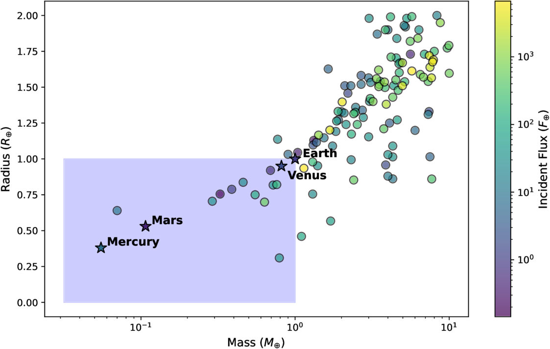
JWST is hunting for atmospheres on small rocky planets around other stars. However, only a select few Mars-like exoplanets have been discovered (Figure 1). This is because sub-Earth planets are small and hard to detect, testing the bounds of current technology. The ones that have been discovered, such as TRAPPIST-1h and Kepler-138b, were detected due to favorable geometry. They happen to orbit very close to a low-mass star or sit in resonant multi-planet systems, which amplify the signal we are looking for. True Mars analogs with low flux and moderate orbital periods remain out of reach. This is precisely what makes Mars itself so important scientifically — it is the only planet of this type we can study up close.

Plot of planetary radius versus planet mass, with symbols colored by incident stellar flux.

Figure 1: A plot of confirmed exoplanets by mass and radius. Most confirmed exoplanets are larger and more massive than Earth. Mars-like planets (dots in the blue box) are rare in confirmed exoplanet detections. [Kane et al. 2026]

Getting to Know Mars, Getting to Know All About Mars

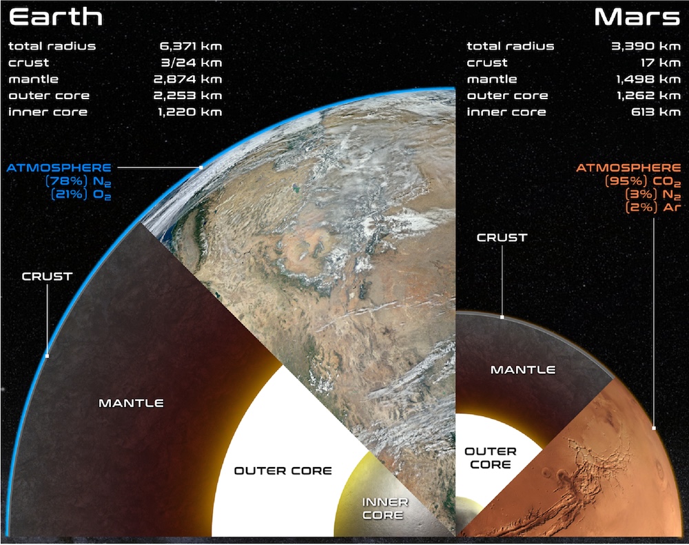
We know a lot about Mars in comparison to other planets thanks to rovers (such as Curiosity and Perseverance), atmospheric orbiters (such as Mars Atmosphere and Volatile EvolutioN and the Mars Orbiter Mission), and other science missions (Figure 2). We know it once had water features with neutral pH and favorable chemistry for life from sedimentary evidence at the Gale and Jezero craters. We know its atmosphere is 95% CO2 with a surface pressure less than 1% of Earth’s. We know it once had an active magnetic dynamo, but the dynamo died out about 4 billion years ago, leading to solar wind steadily stripping away Mars’s atmosphere over time.

Diagram showing Earth and Mars to scale

Figure 2: Earth and Mars to scale, showing their internal structures and atmospheres. Despite being neighbors, Mars is dramatically smaller with a thin CO2 atmosphere, similar to the planets JWST is struggling to characterize. [Kane et al. 2026]

But in the Upside Down, we would know none of this since Mars would be so distant. With current technology, this Upside Down Mars would be essentially undetectable using transit signals, radial velocity measurements, and spectrographs.

Beyond Our Backyard

JWST is currently studying the small rocky TRAPPIST-1 planets and is finding little evidence of atmospheres. The authors of today’s article explore the idea that these exoplanets are similar to Mars and perhaps are undergoing processes that strip away their atmospheres and create optimal conditions for life only for short durations. Using Mars as a blueprint, the authors show how we can better understand exoplanet processes, including volatile delivery and loss, photochemistry, climate evolution, obliquity forcing, planetary architecture, and intrinsic magnetism. For example, measurements of noble gases directly fingerprint Mars’s atmospheric escape process, and the authors argue these give us a calibration framework for interpreting future exoplanet spectra.

The upcoming Nancy Grace Roman Space Telescope’s microlensing survey will start revealing how common true Mars analogs actually are throughout the galaxy, while the future Habitable Worlds Observatory will attempt direct imaging of nearby candidates with unprecedented precision. Together, these missions will tell us whether Mars-like outcomes (brief habitability, catastrophic atmospheric loss, barren surfaces, etc.) are the default fate for small rocky planets. Interpreting that data will require the exact framework this article builds: one grounded in the only Mars analog we can study in detail.

Original astrobite edited by Sandy Chiu.

About the author, Ben Sherwin:

I am a physics PhD student and a National Science Foundation Graduate Research Fellow at Stanford University, working with Josh Frieman. I am interested in theoretical and observational cosmology, specifically in cross-correlations between the cosmic microwave background and tracers of large-scale structure.

The post What if Mars Were a Stranger (Thing)? appeared first on AAS Nova.

Featured Image: A Rare Pair of Galaxies Lacking Dark Matter

20 July 2026 at 17:00

This image, which combines a background view from the Dark Energy Camera Legacy Survey with two inset images from the Very Large Telescope, shows an unusual pair of galaxies in the Fornax Cluster. The galaxies FCC 224 and FCC 240 are under scrutiny because they may have formed via a high-velocity collision between dwarf galaxies — the so-called “bullet-dwarf” model. Using new spectroscopy from the Very Large Telescope, Maria Luísa Buzzo (Yale University) and collaborators analyzed the ages and kinematics of the galaxies’ stars as well as the unusually bright globular clusters swirling around each galaxy. These data suggest that both galaxies are deficient in dark matter, and their stellar populations and globular clusters are all roughly 10 billion years old. The lack of dark matter and the uniform stellar ages are both consistent with the bullet-dwarf model, in which the collision strips away dark matter and ignites a burst of star formation. Since this type of collision can create more than two remnants, the team suggests searching along the trajectory defined by FCC 224 and FCC 240 for more fragments from the collision, some of which may contain the galaxies’ lost dark matter. To learn more about these galaxies and what they might mean for the bullet-dwarf mechanism, be sure to check out the full research article linked below.

Citation

“Dark-Matter-Deficient Twins: FCC 224 and FCC 240 as Possible Analogs of NGC 1052-DF2 and DF4,” Maria Luísa Buzzo et al 2026 ApJ 1005 15. doi:10.3847/1538-4357/ae7349

The post Featured Image: A Rare Pair of Galaxies Lacking Dark Matter appeared first on AAS Nova.

Dating the Dawn of the Milky Way Disk

17 July 2026 at 18:56

Messier 64

The iconic disks of spiral galaxies are well known across the local universe and now far beyond. A recent study looks at the Milky Way to determine when its own disk emerged.

Spinning into Spirals

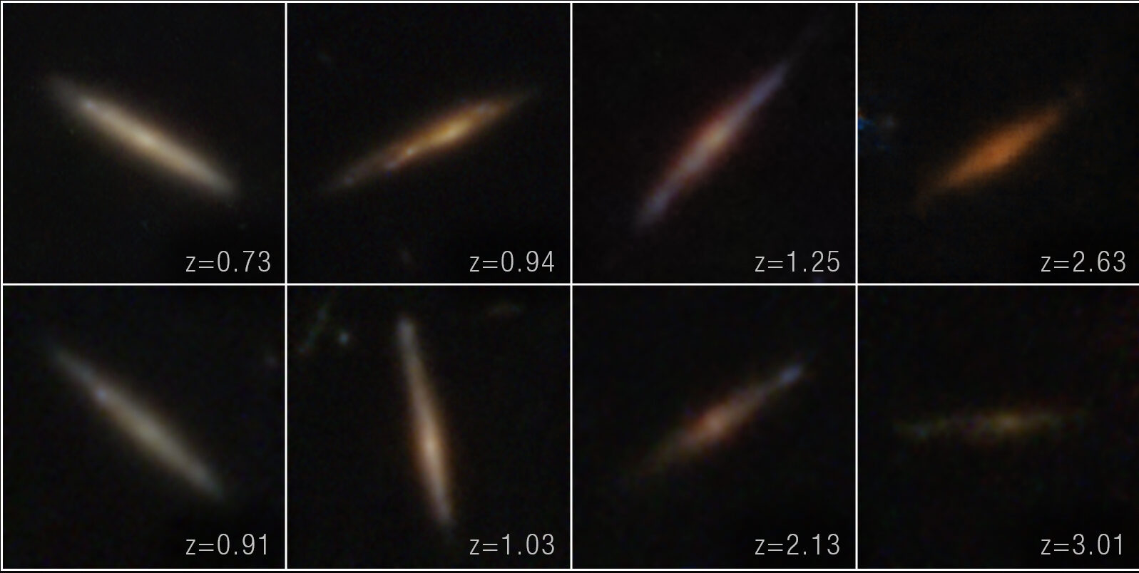
The Milky Way, a grand spiral galaxy with stars and gas rotating in a disk, did not always look this way. Galaxies begin as chaotic clumps of gas and stars inside a knot of dark matter, and at some point in time, spiral galaxies must transform into the flat rotating disks we observe them as today. Recent JWST observations have uncovered disk galaxies emerging much earlier in the universe than previously thought, shifting our understanding of how quickly spiral galaxies come together and settle into disks. While we cannot study the detailed assembly history of these very distant galaxies, we can dissect galaxies in the local universe to build a better timeline of galaxy evolution.

disk galaxies

JWST images of distant edge-on galaxy disks [NASA, ESA, CSA, STScI, Takafumi Tsukui (ANU)]

Looking as close to home as possible, astronomers have used the kinematics and chemical makeup of stars in our own Milky Way to trace the moment when the galaxy started to host a rotating stellar disk. This period, known as the “spin-up,” marks when the bulk kinematic signature of the galaxy transitioned from one dominated by random motions to one dominated by a rotating disk.

Stars hold on to the kinematic and chemical information they are born with, so stars of different ages and metallicities across the galaxy should trace the development of the disk. Because stellar ages have been difficult to constrain observationally, studies of galactic spin-up have typically relied on readily available metallicity measurements as a proxy for age; however, metallicity is not a clear-cut age indicator, making it difficult to truly distinguish different stellar populations across the Milky Way’s disk. Luckily, new major surveys have recently provided stellar databases adding the stellar age measurements necessary to pin down when the Milky Way spun up.

Dawn of the Galactic Disk

Plots showing stellar age and rotational velocity versus metallicity, [Fe/H].

Plots showing stellar age and rotational velocity (Vϕ) versus metallicity, [Fe/H]. The metallicity range where the age–[Fe/H] relation stalls coincides with the point when the Vϕ–[Fe/H] relation rapidly increases, indicating the age of the spin-up in the Milky Way. Click to enlarge. [Modified from Feltzing et al 2026]

Sofia Feltzing (Lund Observatory) and collaborators used a catalog of over 300,000 subgiant stars from the Large Sky Area Multi-Object Fiber Spectroscopic Telescope with metallicities, kinematics, and crucial stellar ages to determine when the Milky Way began to host a stellar disk. After making quality cuts to ensure they included only the most robustly measured stars, the authors divided the sample into two distinct stellar populations that settled into the Milky Way’s disk differently: older stars with a high abundance of α elements (like oxygen, magnesium, and silicon) relative to iron and younger stars with low α-element abundances.

With these star samples, Feltzing and team analyzed how both stellar rotational velocity and age varied with metallicity to determine when the Milky Way spun up. They found that high-α stars clearly move from having random motions to being rotationally supported over a short range of metallicities about 12.5 billion years ago, while the low-α stars seem to begin in a rotating disk and stay there. When varying their selection criteria and looking at the full sample, the authors determined that the Milky Way spin-up happened between 12.1 to 12.5 billion years ago — the first time Milky Way spin-up has been age-dated in this way.

These results imply a rapid chemical evolution and change in kinematic properties as stars went from randomly orbiting to rotating in an ordered disk in the Milky Way. The authors suggest that future studies should focus on lower-metallicity stars to better disentangle stars in the disk from stars in the halo, which will lead to a more precise determination of the Milky Way’s spin-up. Upcoming large-scale surveys will make this possible and allow astronomers to build a better picture of galaxy formation in the early universe.

Citation

“Dawn of the Milky Way Disk: Determination of When a Rotationally Supported Disk Appears and Dating the Spin-up of the Disk,” Sofia Feltzing et al 2026 ApJL 1004 L28. doi:10.3847/2041-8213/ae6f14

The post Dating the Dawn of the Milky Way Disk appeared first on AAS Nova.

Seeking Technosignatures in Polluted White Dwarfs

15 July 2026 at 17:00

white dwarf with debris disk

White dwarfs often show signs of metals in their spectra, providing evidence that these evolved stars have accreted planetary material. Could white dwarf spectra also provide evidence for technological activity in these star systems?

A Record of Planets Past

When a Sun-like star reaches the end of its hydrogen-burning lifetime, it first puffs up into a red giant before exposing its white-hot core, which evolves into a white dwarf. This dramatic transition shakes up any planets that happened to be orbiting the star, and some close-in planets may end up crumbling apart, their rubbly remains peppering the surface of the white dwarf.

So far, astronomers have found hundreds of white dwarfs that appear to be polluted with heavy elements from their destroyed planets. These observations provide a valuable look into the bulk compositions of planetary materials outside our solar system. They may also provide a way to detect patterns of chemical abundances that are not natural, resulting from technological processes like industrial refining or the creation of alloys — in other words, a technosignature that is evidence of not just life, but technologically advanced life.

Seeking Signs of Technology

abundances of meteorites compared to white dwarfs

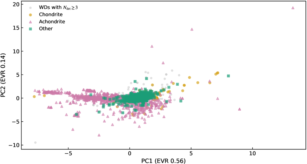
Representation of the chemical abundances of meteorites (pink, orange, and green) and white dwarfs (gray). Most white dwarf abundances overlap with the parameter space defined by the meteorite sample. Click to enlarge. [Huang et al. 2026]

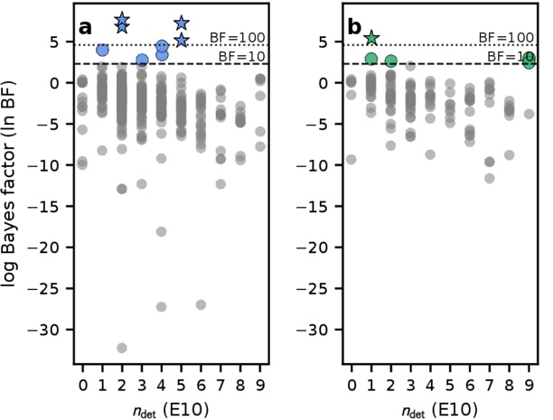
A team led by Bo-Lun Huang (黄博伦) from Beijing Normal University recently investigated whether there is evidence for chemical technosignatures in the current sample of polluted white dwarfs. Huang and collaborators began their investigation with a catalog containing 697 measurements of white dwarfs with metals in their spectra. They applied Bayesian statistical methods to weigh the hypothesis that the chemical makeup of these white dwarfs is entirely natural against the possibility that they contain a blend of natural and technologically altered material.

The team used thousands of chemical abundance measurements from meteorites as a reference for the natural bulk composition of planetary material. For the mixture of natural and processed material, they combined the meteorite reference material with a template that is metal-rich and silicate-poor, with enhanced amounts of iron, nickel, chromium, and manganese.

plot showing evidence for a natural + processed model relative to a natural model as a function of the number of elements detected

Evidence for a model including technologically processed material relative to a purely natural model, as a function of the number of elements detected in the white dwarf. ndet = 0 indicates that only upper limits were obtained on elemental abundances. Higher Bayes factors indicate stronger evidence. The left-hand plot is based on abundances measured from the white dwarfs’ photospheres, while the right-hand plot uses abundances adjusted for diffusion within the white dwarf. Click to enlarge. [Adapted from Huang et al. 2026]

No Strong Evidence, but a Path Forward

Ultimately, Huang’s team found that strong statistical support for the existence of technological processes was uncommon, though there were certain measurements in their sample of white dwarfs that were difficult to reconcile with a solely natural model.

Perhaps unsurprisingly, the team also found that the quality of the chemical abundance measurements affected the constraining power of the observation; some white dwarfs had upper limits for just a few elements, while others had definitive detections of many elements. They found that the most discerning observations recorded iron, magnesium, chromium, and titanium, plus either nickel, silicon, or sodium.

While this work didn’t dredge up firm evidence for technological activity, it provides a jumping-off point for future searches. The handful of white dwarfs in this sample that were fit poorly by a purely natural model could be compared against other technosignature models or targeted with high-resolution spectroscopy. Future measurements of iron and magnesium in polluted white dwarfs may be useful as a preliminary screening tool, helping to pick out intriguing targets for follow-up observations.

Citation

“A Calibrated Bayesian Search for Potential Chemical Technosignatures in Polluted White Dwarfs,” Bo-Lun Huang et al 2026 ApJ 1006 9. doi:10.3847/1538-4357/ae742c

The post Seeking Technosignatures in Polluted White Dwarfs appeared first on AAS Nova.

Can Arid Planets Keep Their Cool?

14 July 2026 at 17:00

side-by-side images of Venus's surface today and an imagining of what its surface might have looked like in the past

Editor’s Note: Astrobites is a graduate-student-run organization that digests astrophysical literature for undergraduate students. As part of the partnership between the AAS and astrobites, we occasionally repost astrobites content here at AAS Nova. We hope you enjoy this post from astrobites; the original can be viewed at astrobites.org.

Title: Carbon Cycle Imbalances on Arid Terrestrial Planets with Implications for Venus
Authors: Haskelle T. White-Gianella and Joshua Krissansen-Totton
Authors’ Institution: University of Washington
Status: Published in PSJ

The Carbon-Cycle Thermostat

When discussing the habitability of planets, we usually focus on the habitable zone, the region around a star where a planet can host a temperature suitable for supporting liquid water on its surface. Yet, being in the right place doesn’t necessarily guarantee that a planet will be habitable.

A planet also needs the right atmospheric composition to sustain the necessary temperatures for hosting liquid water. A key mechanism found on Earth for maintaining this composition is the geologic carbon cycle, which acts as a built-in climate control system. This cycle begins with volcanic eruptions releasing carbon dioxide (CO2), which then dissolves in rainwater and forms a weak acid that weathers rocks on continents. The weathering products wash into oceans, where they form carbonate rocks, locking carbon away. Eventually, plate tectonics recycles some of that carbon back to volcanoes. The weathering process works faster when the planet is warmer, thus regulating the amount of CO2 and stabilizing the climate over long periods of time (but it should be noted that it can take up to a few hundred thousand years to rebalance this slow carbon cycle through the weathering process).

An important caveat is that the weathering process requires sufficient liquid water on the planet’s surface, so what happens in the case for planets with shallower oceans? Low-mass M dwarfs, the most common type of star found in the galaxy, are expected to host less-massive disks and therefore lower water inventories for forming planets. If more “dry” planets are indeed a more likely outcome of planet formation, we’d want to know how their arid conditions influence their long-term evolution and habitability.

Creating Carbon-Tracking Models

The authors built a model that tracks how water and CO2 move between a planet’s interior, oceans, and atmosphere over 4.5 billion years. The model notably includes the following:

  • A sophisticated weathering model that accounts for how runoff can limit rock weathering, improving upon previous models that only included a temperature dependence on weathering
  • Wind-driven evaporation limits that influence the amount of water evaporation in addition to sunlight-driven evaporation
  • Multiple deep water cycle parameterizations that explore how water moves between the interior and the surface

The model tests for four initial surface water inventories (0.1%, 1%, 10%, and 100% of Earth’s oceans) and then simulates how the surface water, atmosphere, and climate evolve over time.

A Critical Water Threshold

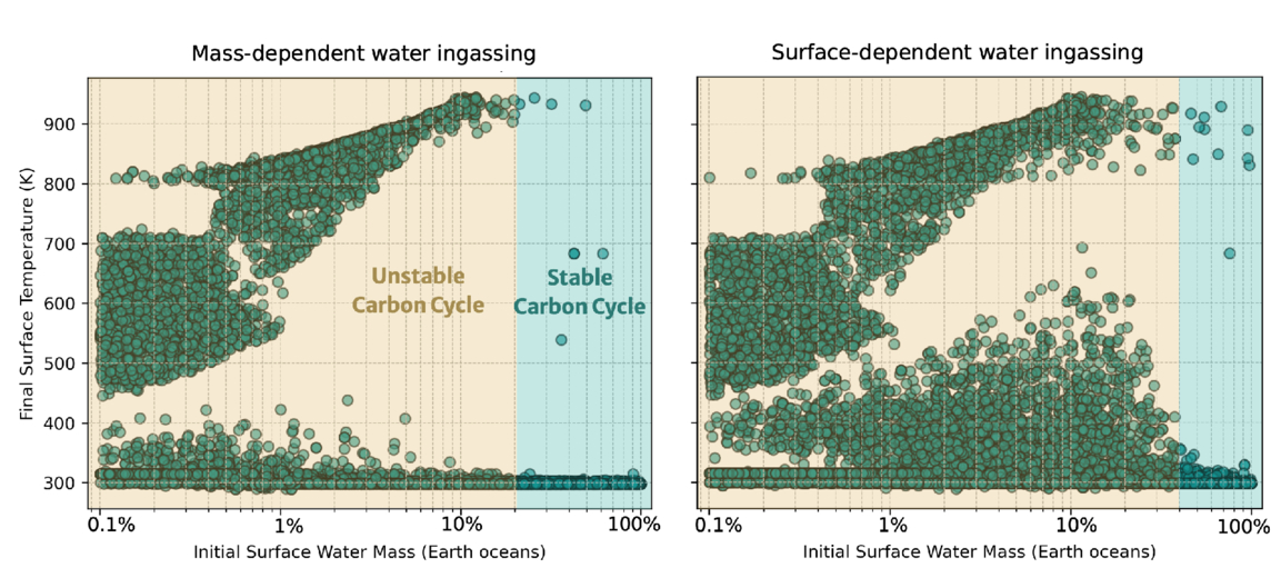
The models reveal that planets require at least 20–50% of Earth’s ocean mass to maintain a balanced carbon cycle. Below this threshold, the carbon cycle becomes unbalanced, leading to devastating consequences for habitability (Figure 1).

two plots of final surface temperature as a function of initial surface water mass

Figure 1: Final surface temperature after simulating 4.5 billion years of evolution as a function of initial water inventory for Earth-like planets. Each dot represents a model run with different assumptions (total carbon inventory, temperature dependence of weathering, soil age, etc.). The yellow region shows where most simulations result in uninhabitable surface temperatures from an unbalanced carbon cycle, and the cyan region shows where most simulations result in habitable surface temperatures and a balanced carbon cycle. The left and right plots show the results for two different parameterizations of the deep water cycle implemented in the model. [White-Gianella & Krissansen-Totton 2026]

For the more arid planets, models reveal a concerning runaway process. Limited surface water reduces precipitation and slows rock weathering. Weathering cannot keep up with volcanic CO2 release, causing CO2 buildup and warming of the atmosphere. The cycle repeats, driving runaway warming until all water evaporates.

Important Implications (Within and Outside Our Solar System)

Looking within the solar system, the results offer an explanation for how a potentially habitable Venus could have transitioned into its current inhospitable state. If Venus had formed with an initial water inventory below this critical threshold of 20–50% of Earth’s ocean mass, then its carbon cycle would have become unbalanced, creating the CO2 inferno seen on Venus today.

In future exoplanet studies, telescopes like the Habitable Worlds Observatory might detect ocean glint (specular reflection from liquid water) or measure land fraction from light curves. Finding a planet in the habitable zone but with limited ocean coverage would likely be bad news, as the planet could be quietly losing its grip on habitability. Astronomers may want to be more careful when looking at seemingly promising planets within their habitable zones.

Original astrobite edited by Natalie Price.

About the author, Jared Bull:

I am a 2nd-year PhD student at Johns Hopkins University. I study brown-dwarf variability and am interested in using time-series observations to uncover dynamic processes within their atmospheres. In my free time I like to read, cook, and do astrophotography.

The post Can Arid Planets Keep Their Cool? appeared first on AAS Nova.

When the Spacecraft Align: Rescuing Saturated Images of Solar Flares

13 July 2026 at 17:00

close-up image of the Sun showing a solar flare

Many observations of solar flares suffer from saturation and blooming, causing crucial information to be lost. Researchers recently validated a technique for retrieving information from saturated flare images, unlocking a treasure trove of powerful solar flares for examination.

Solutions for Saturation

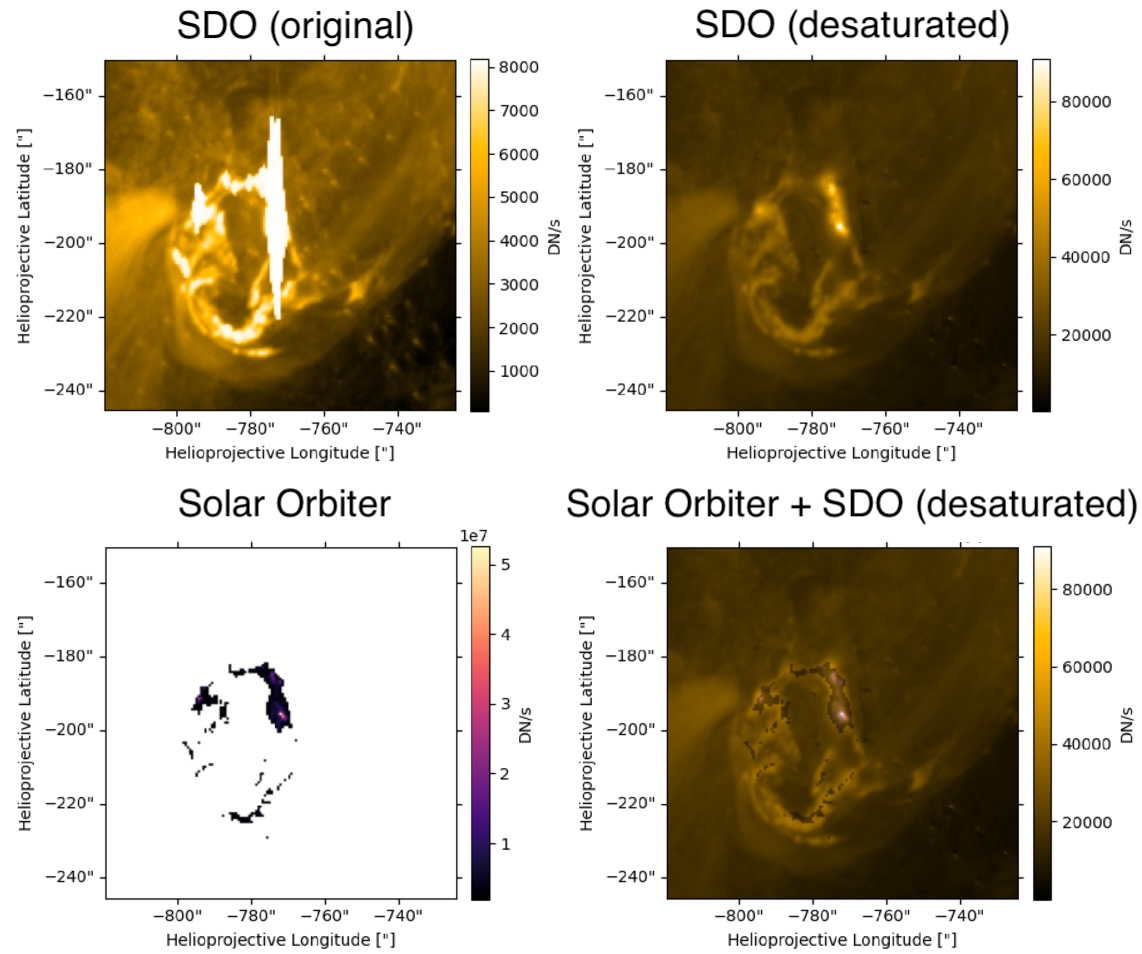
Since 2010, the Atmospheric Imaging Assembly (AIA) on the Solar Dynamics Observatory (SDO) has been capturing nearly continuous extreme-ultraviolet images of the Sun’s disk, revealing our star’s dramatic high-energy behavior. Though SDO/AIA’s observations have transformed our understanding of the Sun’s activity, they have limitations: powerful solar flares can saturate the detector, spilling charge into nearby pixels.

This saturation and overflow compromises our ability to study the most energetic solar flares — but the “lost” information may actually be recoverable. When light from an intense flare enters SDO’s instruments, not all of it pools in the saturated region of the detector: some of the light is diffracted by the optics, and by mathematically inverting this pattern of diffracted light, researchers can attempt to extract the encoded information about the saturated region. Researchers have used this technique for more than a decade, but options for validating the results were limited until now.

Solar Orbiter Lends a Hand

Launched almost 10 years to the day after SDO, the Solar Orbiter spacecraft provides an excellent opportunity to test inversion techniques for recovering information from saturated solar images. Solar Orbiter’s Extreme Ultraviolet Imager snaps brief photos of the Sun at a rapid cadence, and its images remain unsaturated even when faced with energetic solar flares.

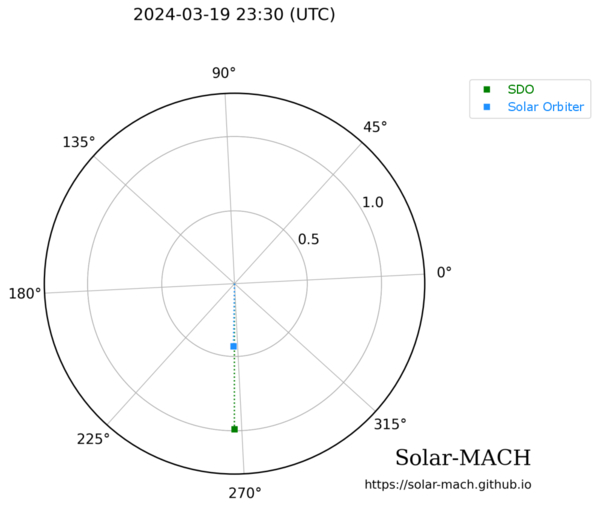
positions of Solar Dynamics Observatory and Solar Orbiter during a solar flare on 19 March 2024

Positions of SDO (green) and Solar Orbiter (blue) during a solar flare on 19 March 2024. Click to enlarge. [Guastavino et al. 2026]

As described in a recent research article by Sabrina Guastavino (University of Genoa; Italian National Institute for Astrophysics) and collaborators, the ideal setup for testing the inversion technique arose on 19 March 2024, when SDO and Solar Orbiter both viewed a solar flare while separated by just 1 degree in longitude.

Guastavino’s team aligned and reprojected the data, accounting for the slightly different viewing angles of the two spacecraft, then applied an algorithm called Adaptive SE-DESAT to reconstruct the flux within the saturated portion of the SDO image. The team compared the desaturated SDO images to the unsaturated Solar Orbiter images over the course of the flare, finding the same flare morphology and similar time evolution between the two data sets.

sample results of the desaturation process

Example of unprocessed SDO data (top left), desaturated SDO data (top right), Solar Orbiter data (bottom left), and a combination of the two data sources (bottom right). Note that the Solar Orbiter observations have been clipped so that only the highest flare intensities were recorded. Click to enlarge. [Adapted from Guastavino et al. 2026]

A Treasure Trove of Desaturated Data

Overall, these results demonstrate the effectiveness of the inversion technique, though Guastavino and coauthors noted that improvements could be made during the impulsive phase of the flare, when the emission is increasing. The team identified several reasons why the results may not match during this phase, including rapid evolution of the flare during individual exposures.

Despite these areas that require further attention, the validation of this technique unlocks 16 years of solar flare observations from SDO. This especially enhances our sample of powerful solar flares, increasing the available records of the most energetic solar flares by orders of magnitude.

Citation

“Validation of an Extreme-Ultraviolet Desaturation Technique for the Atmospheric Imaging Assembly on Board the Solar Dynamics Observatory Using Observations from the Extreme Ultraviolet Imager on Board Solar Orbiter,” Sabrina Guastavino et al 2026 ApJL 1005 L50. doi:10.3847/2041-8213/ae7d2e

The post When the Spacecraft Align: Rescuing Saturated Images of Solar Flares appeared first on AAS Nova.

Putting the Landing Site Before the Lander

10 July 2026 at 17:00

An oblique-angle photograph of a deep crater half in shadow.

NASA is once again sending scientific missions to the Moon. But under the new commercial framework for getting there, researchers need to invent a new method for how to pick where to land.

A New Process for Picking Sites

NASA’s Commercial Lunar Payload Services program is a bold innovation in organizing robotic missions to the Moon. Under this model, rather than keeping the mission process entirely in-house, the agency selects the scientific mission they want to support then simply buys a ride to the lunar surface from a commercial vendor. But, how do you pick a landing site before you know exactly how you’re getting there?

A photograph from orbit of two volcanic mounds on the moon.

The Gruithuisen domes region, the broad area the Lunar-VISE team searched for potential landing sites. Click to enlarge. [Adapted from Williams et al. 2026]

The Lunar Vulkan Imaging and Spectroscopy Explorer (Lunar-VISE) mission, set to launch in mid-2028, was one of the first programs to go through this new landing site selection process. After being officially selected in 2022, the team had just nine months to nail down exactly where their mission should touch down. A recent article led by Jean-Pierre Williams (University of California, Los Angeles) detailed exactly how the team accomplished this task and presented some lessons they learned along the way.

No Parking Lots on the Moon

Picking a landing site is no small task: for context, selecting the landing sites for each of the most recent Mars rovers took five years and multiple community workshops. The Lunar-VISE team therefore took a streamlined and logic-driven approach. They started by explicitly laying out their science objectives: Lunar-VISE’s purpose is to investigate some strangely silicate-rich volcanic formations called the Gruithuisen domes, so they had to land either on or near those. They also had to have access to boulders that were excavated from deep within the domes during a crater formation event, so they had to pick a spot with boulders relatively nearby.

In addition to objectives, they also laid out a slew of constraints. Although they needed boulders nearby, they couldn’t have too many boulders, or any particularly large boulders, since those could pose hazards for landing. There also couldn’t be any steep slopes in the field. Most of the area had to maintain a line of sight with a supporting orbiter for communications, so they couldn’t set down near any ridges. Also, they had to consider how the terrain would cast shadows as the lunar day progressed, since they didn’t want their mission cut short by freezing temperatures and a lack of solar power. As the team quipped, “many interesting, high-science value locations on the Moon may not be in proverbial ‘parking lots.'”

A low-angle photo of a crater and plain on the moon, with arrows and annotations to the landing ellipse, boulders, and the edge of the dome.

An image from the Lunar Reconnaissance Orbiter overlaid onto a terrain model of the final landing site. Click to enlarge. [Williams et al. 2026]

By combing through archival data and working with the team that operates the Lunar Reconnaissance Orbiter Camera, a key asset for making detailed maps of the Moon, the researchers found the perfect spot: alongside a 190-meter-diameter crater named Mareta. This feature is named after Mareta West, one of the first female planetary geologists at the United States Geological Survey and the scientist who selected the landing site for Apollo 11’s historic touchdown.

In addition to presenting their landing site, the researchers offered a handful of lessons to others who may someday be in the fortunate and thrilling position of needing to pick a landing spot on the Moon. For one, they urged teams to coordinate with the Lunar Reconnaissance Orbiter specialists as early as possible, since processing the imaging data for lander-quality maps is a specialized and intensive task. For another, they recommended that all of the software tools used be made publicly available so that future missions don’t need to duplicate their work.

As this article laid out, the Commercial Lunar Payload Services program and Lunar-VISE take us one step closer to making missions to the Moon routine — but we’re still figuring out exactly how to do that.

Citation

“Lunar-VISE Landing Site Selection and Characterization at Mons Gruithuisen Gamma,” Jean-Pierre Williams et al 2026 Planet. Sci. J. 7 161. doi:10.3847/PSJ/ae7d2c

The post Putting the Landing Site Before the Lander appeared first on AAS Nova.

Gaia Data Show That the Initial Mass Function Is Not Universal

8 July 2026 at 22:48

star-forming cloud OMC-2

Do all star-forming regions birth stars with the same distribution of masses? Theory suggests that they do not, but researchers often assume they do for simplicity. Now, ultra-precise observations from Gaia have demonstrated that the initial mass function varies across star clusters in the Milky Way.

A Universal Initial Mass Function?

JWST image of galaxies in the iconic Hubble Ultra Deep Field

The light from distant galaxies is dominated by high-mass stars, requiring the use of the IMF to estimate the stellar mass of a galaxy. [ESA/Webb, NASA & CSA, G. Östlin, P. G. Perez-Gonzalez, J. Melinder, the JADES Collaboration, the MIDIS collaboration, M. Zamani (ESA/Webb); CC BY 4.0]

When a molecular cloud fragments, collapses, and births a star cluster, how many stars form, and what are their masses? The answer to that question is what astronomers term the initial mass function, or IMF: the distribution of masses of stars born in a cluster.

The IMF is important in many areas of astronomy, and it’s relied on especially heavily in studies of distant galaxies. The light from these galaxies is dominated by high-mass stars, with the emission from lower-mass stars lost in the glare, so astronomers must use the IMF to reconstruct the stellar populations of these far-off locales.

Though theory suggests that the IMF should vary with factors like temperature and metallicity, demonstrating these variations has been difficult, even within our own galaxy. Because of this, researchers often adopt a universal IMF drawn from observations of star clusters in the Milky Way. But is the IMF truly universal?

The More the Slope Changes, the More the Break Mass Stays the Same

Determining whether the IMF is universal is more complicated than simply comparing the stars in one cluster to those in another. That’s because what astronomers measure in present-day star clusters is not the initial mass function, but a version of the IMF that has been skewed by millions to billions of years of evolution; over time, high-mass stars die and low-mass stars get ejected, warping the shape of the mass function.

Plots of the stellar mass function

Left: Different break masses arise for different properties (here, the sound speed) of a given star-forming cloud. Right: Evolution of the mass function over time for a single star cluster. Over time, high-mass stars die and low-mass stars are ejected from the cluster, resulting in a decrease in the remaining mass fraction, μ, from 1 to 0.1. The slopes change, but the break mass does not. Click to enlarge. [Adapted from Steinhardt et al. 2026]

However, as demonstrated in a recent research article led by Charles L. Steinhardt (University of Missouri), certain aspects of the IMF may remain unchanged as clusters evolve. When the mass function of a star cluster is described using a broken power law (commonly called a “Kroupa-like” IMF in reference to work by Pavel Kroupa), the slopes of the power-law segments are affected by stellar evolution and dynamical interactions. Crucially, these effects appear not to alter the break mass — the mass at which the IMF transitions from one slope to another. Therefore, differences in the break mass from cluster to cluster reflect differences in the underlying IMF rather than the stellar and dynamical evolution of the clusters.

Insights from Gaia

Thanks to the Gaia spacecraft, which made precise observations of more than 2 billion stars in the Milky Way and beyond, it’s now possible to measure and compare the break masses of individual star clusters. Out of an initial catalog of 7,167 Milky Way clusters observed with Gaia, Steinhardt’s team selected just 110 that were of high enough quality and contained a sufficient number of stars to measure cluster break masses accurately.

Plot of stellar mass function for four Milky Way clusters

Observed mass functions of four Milky Way star clusters. The break masses are clearly different, showing that the IMF must vary from cluster to cluster. Click to enlarge. [Steinhardt et al. 2026]

The team found that the break mass differs considerably between the clusters in their sample, showing that the IMF is not universal. The observed variety of break masses appears to be linked to the age of the cluster, but instead of reflecting the impact of stellar and dynamical evolution — which have no effect on the break mass — these differences reflect the properties of the clouds in which the clusters were born. This implies that the properties of star-forming clouds in the Milky Way have, on average, changed over cosmic time. Thus, a star cluster that formed billions of years ago would have had a different IMF than one forming today.

This finding has implications for studies of high-redshift galaxies, where the properties of star-forming clouds are markedly different from those in the Milky Way. Going forward, Steinhardt and coauthors recommend developing a flexible parameterization of the IMF to capture how this critical function behaves in environments vastly different from our own.

Citation

“Direct Evidence for Stellar Initial Mass Function Variation in the Milky Way,” Charles L. Steinhardt et al 2026 ApJL 1005 L40. doi:10.3847/2041-8213/ae7444

The post Gaia Data Show That the Initial Mass Function Is Not Universal appeared first on AAS Nova.

Distant Galaxies: Dead or in Disguise?

7 July 2026 at 17:00

distant starburst galaxies

Editor’s Note: Astrobites is a graduate-student-run organization that digests astrophysical literature for undergraduate students. As part of the partnership between the AAS and astrobites, we occasionally repost astrobites content here at AAS Nova. We hope you enjoy this post from astrobites; the original can be viewed at astrobites.org.

Title: MAGAZ3NE: Confirming Dust Deficiency and Quiescent Nature of Ultramassive Galaxies at 3 < z < 4 with ALMA Observations
Authors: Wenjun Chang et al.
First Author’s Institution: University of California, Riverside
Status: Published in ApJ

Distant galaxies offer a unique window into how stars, gas, and dust evolve over cosmic time. Tracing this evolution requires understanding not only how galaxies form, but also how and when they stop forming stars, a process known as quenching. Understanding how, when, and why galaxies quench is a fundamental question in astrophysics, and one that requires observations of star-forming, quenching, and fully quenched galaxies alike. Unfortunately, one complication is that identifying truly quenched galaxies is challenging: galaxies that appear “dead” may instead be actively forming stars, hidden behind a thick veil of dust.

In today’s article, the authors use observations from the Atacama Large Millimetre/submillimetre Array (ALMA) to investigate five ultramassive galaxies at redshifts, z, between 3 and 4, and ask a deceptively simple question: are these massive red galaxies genuinely quenched, or are they secretly forming stars behind the scenes?

Meet the Suspects: Ultramassive Galaxies at the Edge of Cosmic Noon

The five galaxies in this study are drawn from the Massive Ancient Galaxies at z > 3 NEar-infrared (MAGAZ3NE) survey, which targets some of the most massive galaxies known at early cosmic times. All five have stellar masses exceeding 100 billion solar masses and have been confirmed at z > 3. At these redshifts, we are observing the galaxies as they were when the universe was less than 2 billion years old. This is just before an epoch known as cosmic noon, when star formation across the universe reached its peak.

These galaxies also benefit from extensive multiwavelength observations from a range of observatories, including the ground-based Visible and Infrared Survey Telescope for Astronomy and the Spitzer Space Telescope. By combining imaging across wavelengths from the ultraviolet to the near-infrared, astronomers can measure the “colours” of galaxies and use these colours to infer the galaxies’ star-forming activity.

Galaxies that have quenched their star formation are dominated by older stellar populations, which makes them appear red (hence why they are often referred to as “red and dead” galaxies). However, dust can redden galaxies in a similar way by absorbing blue light and re-emitting it at longer wavelengths — meaning that a dusty, star-forming galaxy can easily masquerade as a quenched one. To uncover any hidden star formation, the authors turn to ALMA to search for far-infrared dust emission. The sample of galaxies investigated with ALMA is shown in Figure 1.

UVJ color–color diagram

Figure 1: UVJ colour–colour diagram, which uses galaxy colours in the ultraviolet (U), visible (V), and near-infrared (J) to identify quenched galaxies. The five ultramassive galaxies (UMGs) studied here (filled cyan circles) lie firmly in the quenched region (QG), consistent with a lack of ongoing star formation. Crosses indicate galaxies undetected in ALMA dust emission, while other massive galaxies at similar redshifts are shown in grey for comparison. [Chang et al. 2026]

ALMA on the Scene

ALMA observes light at sub-millimetre wavelengths, which at these redshifts traces emission from star-forming regions that are obscured by dust. Of the five ultramassive galaxies in this sample, only one is detected with ALMA. Even when the remaining four galaxies are stacked together, no dust emission is recovered, indicating that if any dust is present, it must be extremely faint.

To better quantify what these ALMA non-detections imply, the authors perform spectral energy distribution fitting (see a recent overview bite on spectral energy distribution fitting) using the Code Investigating GALaxy Emission, or CIGALE, a code that enforces energy balance between absorbed starlight and dust emission to estimate physical properties such as a galaxy’s star formation rate and dust content. With the ALMA constraints included, all five galaxies are found to lie more than 10 times below the star-forming main sequence. Even the single ALMA-detected galaxy remains formally quenched, showing only weak residual star formation.

In other words, these galaxies really are dead (or at least extremely dormant).

Extremely Dust-Poor Galaxies

The spectral energy distribution fitting also allows the authors to measure how much dust these galaxies contain relative to their stellar mass. This ratio provides a simple but powerful way to assess how much interstellar material remains in a galaxy — and therefore how much fuel is left for future star formation.

Three of the five ultramassive galaxies have ratios of Mdust/Mstar < 10-4 (Figure 2), placing them among the most dust-poor quenched galaxies confirmed at z > 3. The lone galaxy detected by ALMA contains slightly more dust, with Mdust/Mstar = 10-3, but even this is far below what would be expected for an actively star-forming galaxy. For comparison, typical star-forming galaxies at similar stellar masses host more than 100 times more dust.

Plot of dust-to-stellar mass ratio versus redshift

Figure 2: The ratio of dust mass to stellar mass versus redshift for massive quenched galaxies (QGs). This quantity measures how dust rich a galaxy is compared to its stellar mass. The ultramassive galaxies in this study (cyan pentagons) fall well below the dust content expected for star-forming galaxies (solid blue line), highlighting their extreme dust deficiency. [Adapted from Chang et al. 2026]

These results raise important questions about how galaxies can become ultramassive, quenched, and nearly dust-free within the first two billion years of cosmic history.

For now, ALMA has delivered a clear answer to the question of “dead or in disguise?”: at least some candidate ultramassive galaxies in the early universe really are quenched, and they are strikingly dust poor. By ruling out the dusty impostor scenario, this study shows that deep ALMA observations can cleanly distinguish genuinely quenched galaxies from dusty star-forming ones, even at the highest stellar masses and earliest cosmic times. How these galaxies lost their dust remains an open question, but one thing is clear: by the time cosmic noon arrived, some galaxies had already finished forming stars and quietly faded into dormancy.

Original astrobite edited by Viviana Cáceres.

About the author, Lucie Rowland:

I’m a fourth (and final!) year PhD student at Leiden Observatory in the Netherlands, studying massive, star forming galaxies in the early universe with ALMA and JWST. It’s a really exciting time to be interested in astronomy, so I hope to make groundbreaking new research more accessible!

The post Distant Galaxies: Dead or in Disguise? appeared first on AAS Nova.

Featured Image: A Mass Mystery in the Bullet Cluster

6 July 2026 at 17:00

Bullet Cluster with mass countours

The Bullet Cluster is best known for being considered a “smoking gun” for the existence of dark matter, but even a famous galaxy cluster like this one has its secrets. For more than two decades, different measurements of the merging clusters’ dynamical mass ratio have yielded vastly different results. In a recent research article, Boseong Young Cho (Yonsei University) and collaborators used data from JWST and the Dark Energy Camera to revisit the Bullet Cluster and measure its mass ratio using new data. The image above shows a near-infrared view of the Bullet Cluster from JWST, with an overlay of mass contours derived from gravitational-lensing measurements. The team’s analysis assigned a mass of 1.5 quadrillion solar masses for the main cluster (on the left side of the image above), and a mass of 150 trillion solar masses for the subcluster. This suggests a mass ratio of roughly 10, which matches the value supported by hydrodynamical simulations and cements the event as a minor merger. The team also identified three distinct cluster halos (two in the main cluster and one in the subcluster), providing an important constraint on the cluster configuration for future modeling. To learn more about this investigation of the Bullet Cluster, be sure to check out the full research article linked below!

Citation

“Joint JWST–DECam Lensing Reveals that the Bullet Cluster Is a Minor Merger,” Boseong Young Cho et al 2026 ApJ 1005 28. doi:10.3847/1538-4357/ae6a90

The post Featured Image: A Mass Mystery in the Bullet Cluster appeared first on AAS Nova.

❌