❌

Normal view

Low Water at San Carlos Reservoir

17 June 2026 at 05:01
June 7, 2023
May 22, 2026
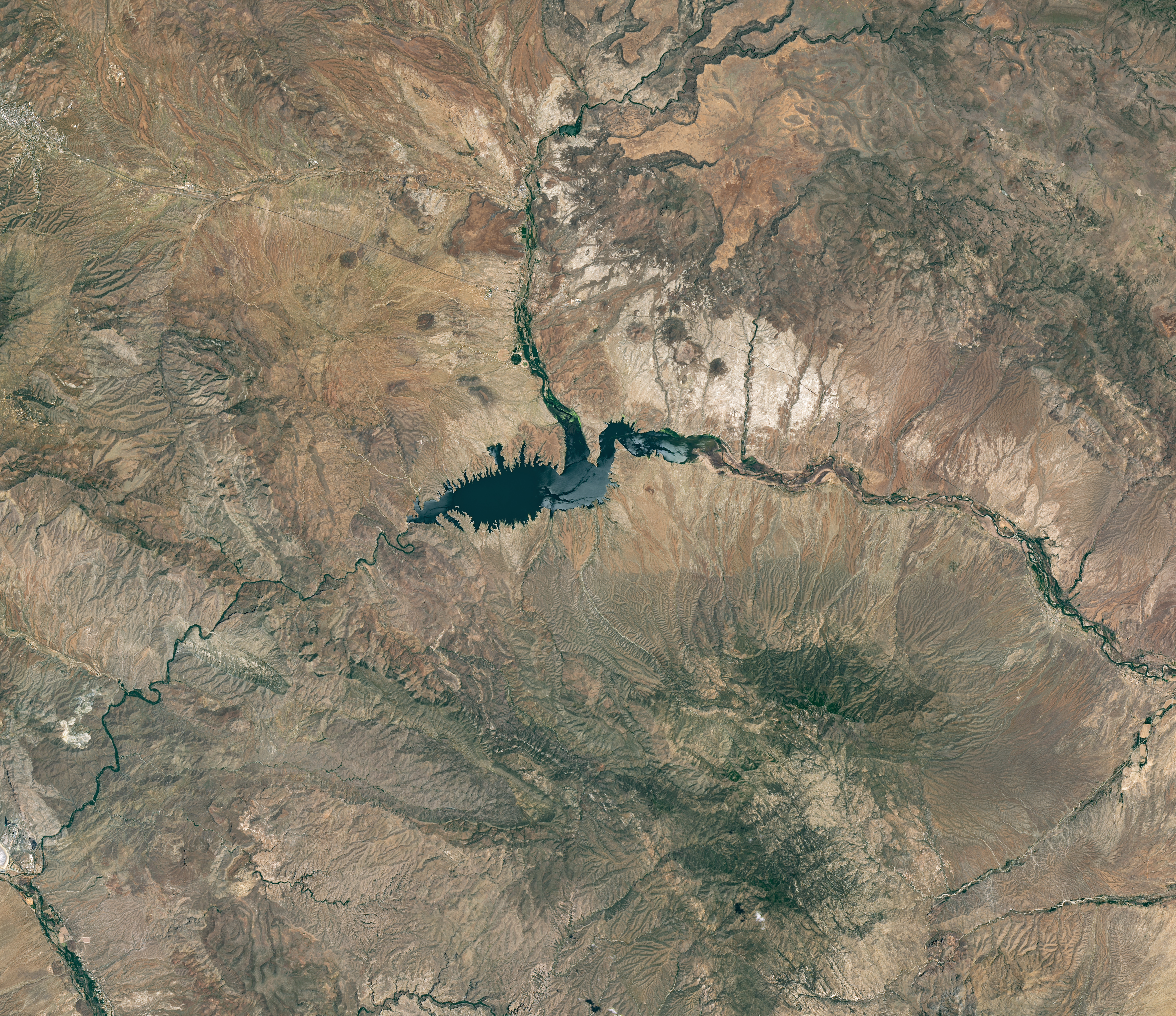
The reservoir appears lake-like and expansive in an image acquired in June 2023.
NASA Earth Observatory/Michala Garrison
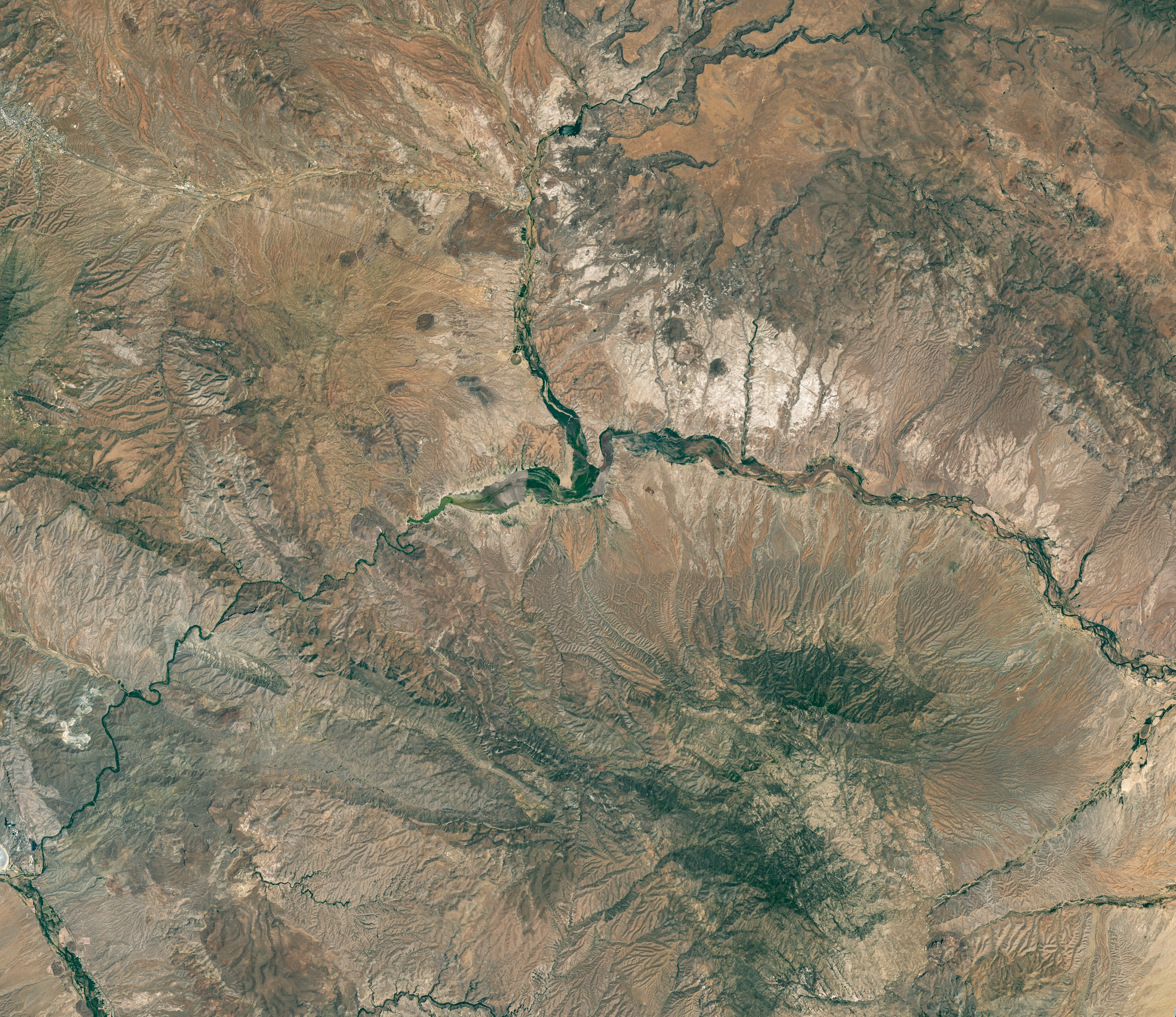
The reservoir is nearly empty by May 2026. The Gila River's natural channel is now visible and flanked with green vegetation in what had been the bottom of the reservoir.
The reservoir is nearly empty by May 2026. The Gila River’s natural channel is now visible and flanked with green vegetation in what had been the bottom of the reservoir.
NASA Earth Observatory/Michala Garrison
June 7, 2023
May 22, 2026
Little water remains in the San Carlos Reservoir in May 2026 (right) compared to fuller conditions in June 2023 (left). Images were captured by the OLI (Operational Land Imager) on the Landsat 9 and 8 satellites, respectively. NASA Earth Observatory images by Michala Garrison.

The Gila River is among the Southwest’s most important rivers, delivering water for people, farms, and wildlife while linking the snow-fed mountains of southwestern New Mexico to the desert lowlands of southwestern Arizona.

In wetter years, seasonal snowfall on the Mogollon Mountains and Black Range provides much of the river’s spring flow and helps refill San Carlos Reservoir, which is formed by the Coolidge Dam. When filled to capacity, the reservoir is one of Arizona’s largest bodies of water.

However, in 2026, lackluster snowfall left the mountain snowpack in the Gila River watershed at 2 percent of the 1991-2020 March median. The limited snowpack pushed April streamflow to 39 percent of normal. By June, after mandatory water releases for downstream agriculture, the reservoir held less than 400 acre-feet of water.

The Landsat image above (right) shows the near-empty reservoir on May 22, 2026, when it stored 389 acre-feet of water—less than 1 percent full; the other image (left) shows the same area in June 2023, when it was about 60 percent full. The green vegetation growing along the river channel and reservoir edge includes a mixture of tamarisk, willow, cottonwood, sedges, and grasses.

Officials closed the reservoir indefinitely on June 5, 2026, after the declining water levels contributed to low oxygen levels—hypoxia—that killed virtually all of its fish. Species living in the reservoir included largemouth bass, black crappie, bluegill, channel catfish, flathead catfish, and several stocked species, including brown trout and rainbow trout. The decomposing fish may pose health risks to people attempting to boat or fish, the San Carlos Recreation and Wildlife Department warned.

The reservoir has hit similarly low water levels in the past, running out of water at least 20 times since it was filled in 1930, according to news reports. Even when the dam and reservoir were first dedicated, there was enough grass growing on the dried reservoir bottom that humorist Will Rogers famously quipped to President Calvin Coolidge: “If that was my lake, I’d mow it.”

Other years with major fish kills include 1976 and 2018. After more than 5 million fish died during a similar event in 1976, the Gila Herald reported that it took five years for the lake’s ecosystem to rebound.

The region is currently in the midst of a multi-year dry period that has left much of the Gila River’s headwaters in New Mexico in a state of severe drought, according to data from the U.S. Drought Monitor.

However, the river’s flow is highly variable, and heavy rains during the coming wet season could help the reservoir recover. A seasonal monsoon outlook released by NOAA in May 2026 projected a 33 to 50 percent chance that an above-average amount of rain would fall in the region that summer. El Niño in the central and eastern equatorial Pacific, which was strengthening in late spring 2026, can make heavy rains in the U.S. Southwest more likely.

NASA Earth Observatory images by Michala Garrison, using Landsat data from the U.S. Geological Survey. Story by Adam Voiland.

Downloads

The reservoir appears lake-like and expansive in an image acquired in June 2023.

June 7, 2023

JPEG (16.60 MB)

The reservoir is nearly empty by May 2026. The Gila River's natural channel is now visible and flanked with green vegetation in what had been the bottom of the reservoir.

May 22, 2026

JPEG (16.85 MB)

References & Resources

You may also be interested in:

Stay up-to-date with the latest content from NASA as we explore the universe and discover more about our home planet.

Drought Parches Florida
4 min read

The state was unusually dry for much of 2025, but the intensity of the drought has ratcheted up since January…

Article
Snow Is Scarce in the Upper Colorado Basin
5 min read

The mountains of Utah and Colorado are among the areas of the western U.S. that are low on snow and…

Article
Spring Rains Saturate Michigan
3 min read

Above-normal precipitation has swollen rivers and damaged infrastructure statewide.

Article

The post Low Water at San Carlos Reservoir appeared first on NASA Science.

Air Pollution’s Daily Pulse Over the Northeast

11 June 2026 at 05:01
7:05 am
3:05 pm
A map of morning nitrogen dioxide shows elevated concentrations of the gas over a region stretching from New York City to Washington, D.C., at 7:05 a.m. on May 18, 2026. A second map of the same area shows much lower concentrations that afternoon.
TEMPO detected high concentrations of nitrogen dioxide during the morning commute at 7:05 a.m. local time on May 18, 2026 (left), along the New York-Washington corridor. The instrument detected lower levels of the gas at 3:05 p.m. (right), after chemical reactions involving nitrogen dioxide had contributed to elevated ozone concentrations in the afternoon.
NASA Earth Observatory/Michala Garrison
7:05 am
3:05 pm
TEMPO detected high concentrations of nitrogen dioxide during the morning commute at 7:05 a.m. local time on May 18, 2026 (left), along the New York-Washington corridor.The instrument detected lower levels of the gas at 3:05 p.m. EDT (right), after chemical reactions involving nitrogen dioxide had contributed to elevated ozone concentrations in the afternoon. NASA Earth Observatory images by Michala Garrison.

More than 35 million people live along the New York–Washington corridor and breathe the region’s air. While air quality has improved significantly in recent decades, outbreaks of ground-level ozone remain common, particularly in the warm summer months, when the chemical reactions that produce the pollutant accelerate and stagnant air allows ozone to accumulate.

A reminder of this seasonal phenomenon came earlier than usual in 2026, when a mid-May heat wave prompted the New York State Department of Health and the New York Department of Environmental Conservation to issue a health advisory on May 17 over concerns about ozone. The code orange advisory warned young people, older adults, and those working or exercising outdoors to limit activity due to ozone’s respiratory and cardiovascular health impacts.

As expected, ground-based air-quality sensors operated by state and federal agencies showed ozone reaching unhealthy levels for sensitive groups on May 18, something that typically happens several times per year. Meanwhile, NASA’s TEMPO (Tropospheric Emissions: Monitoring of Pollution) instrument observed the event from geostationary orbit 22,000 miles (35,000 kilometers) above the equator, a unique vantage point that allows the sensor to collect frequent observations of air pollution.

TEMPO detects nitrogen dioxide (NO2), a gas emitted by burning fuels, particularly by motor vehicles, that contributes to ozone formation. “There’s often a clear and interesting pattern in TEMPO’s nitrogen dioxide data during ozone alert days,” said Hazem Mahmoud, an atmospheric scientist at NASA’s Atmospheric Science Data Center at Langley Research Center. “We see high concentrations of nitrogen dioxide during the early morning commute that drop off sharply in the late afternoon as ozone increases.”

The decline occurs as sunlight fuels photochemical reactions involving nitrogen dioxide, volatile organic compounds, and oxygen that lead to ozone formation. By late afternoon, these reactions deplete much of the available nitrogen dioxide, slowing ozone production until the cycle begins again the next day.

The pair of images above underscores the pattern. The image on the left was acquired at 7:05 a.m. local time when nitrogen dioxide concentrations were high during the morning commute. By 3:05 p.m. (right), most of the nitrogen dioxide had declined substantially, and surface ozone levels were elevated (below). Meanwhile, afternoon sea breezes appear to have transported the remaining nitrogen dioxide slightly to the west. Note that the data shown is provisional, and processing methods are still being refined.

Sensors on earlier polar-orbiting satellites, such as OMI (Ozone Monitoring Instrument) and TROPOMI (Tropospheric Monitoring Instrument), sampled nitrogen dioxide over New York once per day. After its launch in 2023, TEMPO began providing data every hour, allowing researchers to track the evolution and dispersion of air pollution at much finer time scales. 

“TEMPO is helping fill data gaps between ground stations and allowing us to ask new questions,” Mahmoud said. The mission provides data that can improve not only air quality forecasts during crisis situations, such as wildfires, but also the atmospheric models used to forecast the daily rhythms of urban pollution. Such models help researchers understand how natural factors such as winds, humidity levels, and air temperatures influence pollution plumes over the course of a day.

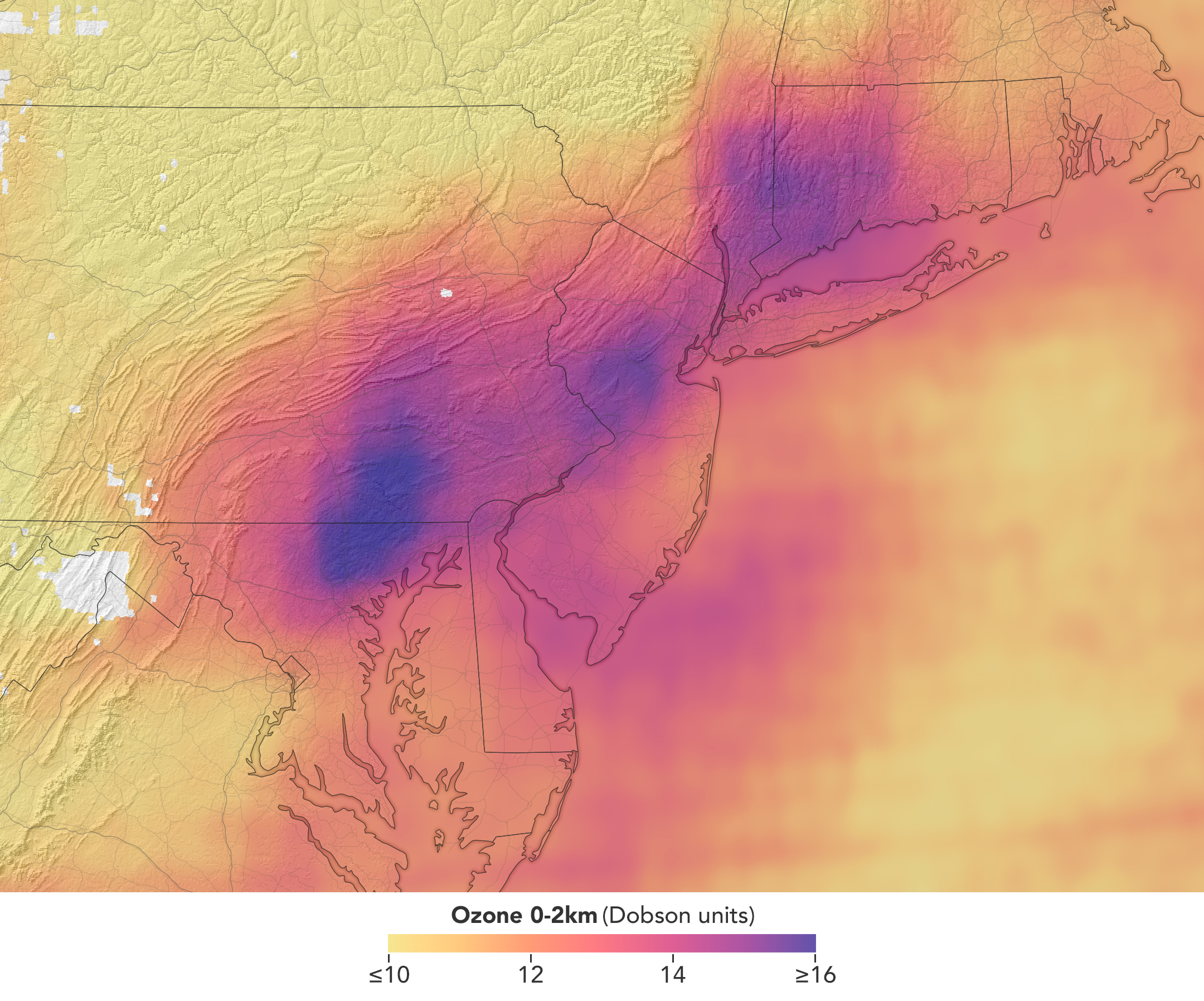
In a map of the eastern U.S., elevated ozone concentrations appear as a purple patch in an area extending from New York City to Washington, D.C.
TEMPO detected elevated ozone concentrations in an area extending from New York City to Washington, D.C., at 5:05 p.m. on May 18, 2026.
NASA Earth Observatory/Michala Garrison

TEMPO also detects ozone directly, but determining how much of that ozone is near the surface versus higher in the atmosphere can be challenging. Most of Earth’s ozone resides in the stratosphere, well above the troposphere, where people live and breathe. At times, however, stratospheric ozone can be transported downward into the troposphere. During events known as stratospheric intrusions, it can even descend far enough to affect air quality at the surface and add to the ozone produced at ground level.

By combining TEMPO observations with other sources of information, researchers are studying the processes that influence the distribution of ozone vertically in the atmosphere. On May 18, NASA’s ground-based tropospheric lidar network (TOLNet) in New York City recorded high concentrations of ozone near the surface, indicating that TEMPO was detecting mostly surface-level ozone associated with urban emissions and not ozone aloft, said Mahmoud.

However, on May 19, the same sensor observed a layer of ozone descending from above 5 kilometers (3 miles), he added, a clue that some of the ozone TEMPO detected that day may have originated in the stratosphere. “This is the type of information that leads to better air quality forecast models and more accurate alerts,” Mahmoud said. “Alerts can affect tens of millions of people and lead to disruptions in school, sports, and other activities, so it’s essential that they be as accurate as possible.”

On June 6, New York authorities issued another health advisory for ozone. People interested in following the event can access daily near-real-time TEMPO observations of ozone, nitrogen dioxide, and other gases on NASA’s Worldview browser, on an interactive Harvard & Smithsonian Center for Astrophysics browsing tool, and on NASA’s Earthdata portal.   

NASA Earth Observatory images by Michala Garrison, using TEMPO data from NASA Earthdata. Story by Adam Voiland.

Downloads

A map of morning nitrogen dioxide shows elevated concentrations of the gas over a region stretching from New York City to Washington, D.C., at 7:05 a.m. on May 18, 2026. A second map of the same area shows much lower concentrations that afternoon.

Nitrogen Dioxide – May 18, 2026 7:05 AM EDT

JPEG (2.52 MB)

A map of morning nitrogen dioxide shows elevated concentrations of the gas over a region stretching from New York City to Washington, D.C., at 7:05 a.m. on May 18, 2026. A second map of the same area shows much lower concentrations that afternoon.

Nitrogen Dioxide – May 18, 2026 3:05 PM EDT

JPEG (2.25 MB)

In a map of the eastern U.S., elevated ozone concentrations appear as a purple patch in an area extending from New York City to Washington, D.C.

Ozone – May 18, 2026 5:05 PM EDT

JPEG (2.10 MB)

References & Resources

You may also be interested in:

Stay up-to-date with the latest content from NASA as we explore the universe and discover more about our home planet.

Smoke Shrouds Northern Thailand
3 min read

Seasonal fires have darkened skies over Southeast Asia.

Article
Winter’s End Is Written in the Clouds
3 min read

As winter turned to spring, the skies over the Gulf of Alaska displayed textbook examples of numerous cloud formations.

Article
Extreme January Cold
3 min read

Following a significant winter storm, frigid temperatures lingered in late January 2026 across a vast swath of the U.S.

Article

The post Air Pollution’s Daily Pulse Over the Northeast appeared first on NASA Science.

Tyndall’s Trail of Bergs

10 June 2026 at 05:01
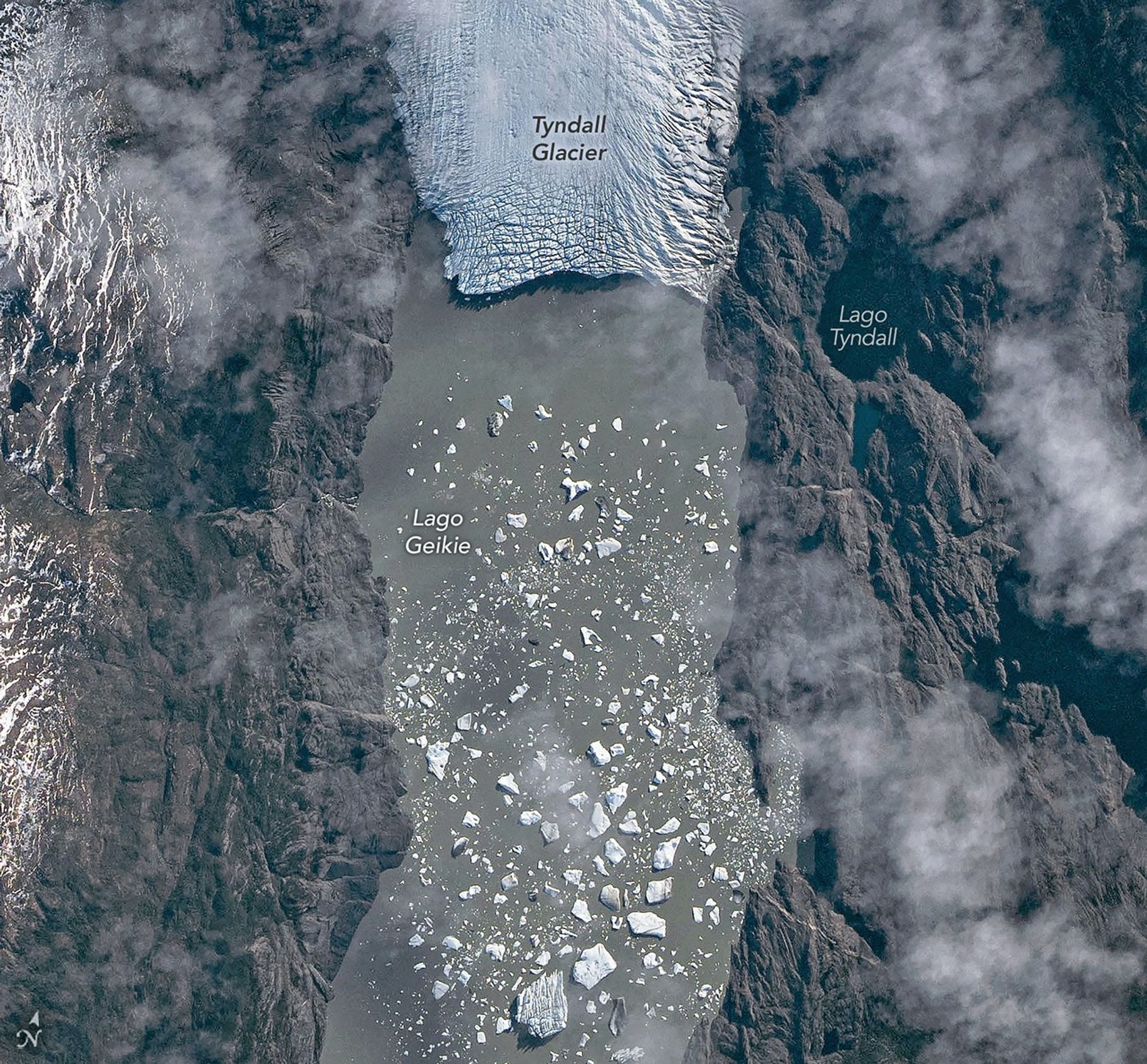
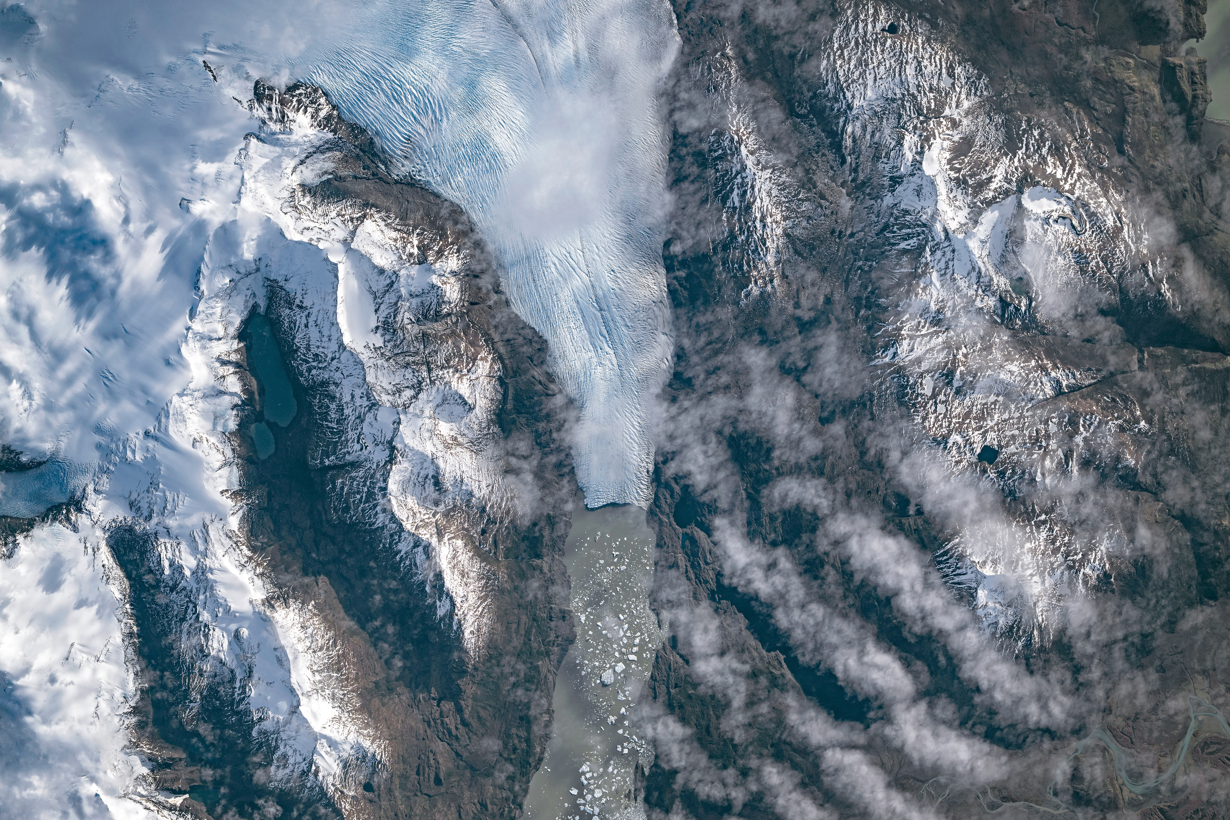
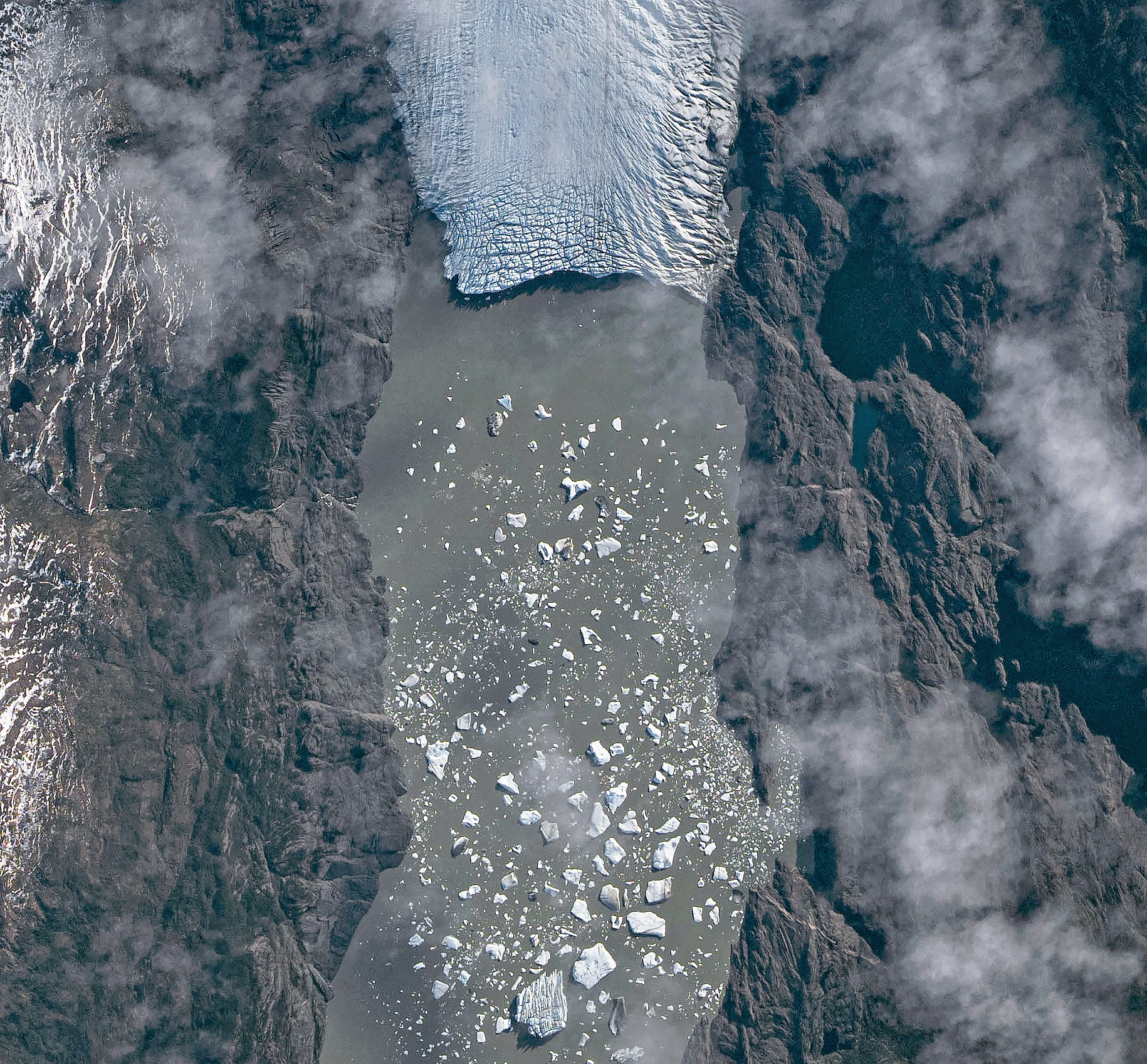
A top-down photo shows a glacier running from north to south amid snowy, mountainous terrain. The glacier flows into a narrow lake where many small icebergs are visible floating on the water.
May 10, 2026

The Southern Patagonian Icefield is the largest expanse of ice in the Southern Hemisphere outside of Antarctica. The mass of glacial ice extends hundreds of kilometers along the spine of the Andes, feeding dozens of dynamic outlet glaciers that grind their way down from higher elevations. Many of these rivers of ice terminate in the sea or in proglacial lakes.

An astronaut aboard the International Space Station photographed one of these glaciers—Tyndall Glacier in southern Chile—through a layer of ethereal clouds on May 10, 2026. Fragments of ice that had calved off its terminus were visible floating on Lago Geikie.

Like most Patagonian glaciers, Tyndall has been shrinking since the end of the Little Ice Age about 150 years ago. Lago Geikie formed at Tyndall’s terminus around 1940, according to glaciologist Mauri Pelto of Nichols College, and gradually expanded as the ice retreated. Part of the glacier previously terminated in Lago Tyndall to the east, but thinning ice cut off that outlet by 2010, Pelto said. (The ice’s retreat also exposed bedrock along its eastern edge that contains scores of ichthyosaur fossils.)

Along with thinning, ice calving off the glacier’s front has reduced its volume. Tyndall has lost 2.2 kilometers (1.4 miles) in length since November 2022, Pelto said, following about a decade of limited retreat with considerable thinning. A significant calving event in March and April 2023 contributed to the recent uptick in ice retreat. During that time, satellites observed several large icebergs breaking away from Tyndall’s terminus.

Austral autumn in 2026 was a time of active calving retreat at Tyndall (and some neighboring glaciers), Pelto said, albeit more incremental than three years prior. “The substantial crevasses crisscrossing the glacier near the calving front lead to many smaller icebergs,” he said. On the other hand, larger tabular icebergs tend to form when there are fewer deep crevasses near the terminus and the glacier’s ice is thinner.

A top-down photo shows a detailed view of the leading edge of a glacier terminating in a lake. The glacial ice is heavily crevassed with intersecting linear features.
May 10, 2026

The ice cliff at the terminus casts a substantial shadow, which can help scientists estimate the height of the glacier’s front. Pelto’s calculations, using information about the Sun’s position provided with the image, indicate that Tyndall’s front loomed 30–40 meters (100–130 feet) above the lake surface in May 2026. Observations from orbit, including astronaut photographs, can help scientists monitor and understand glaciers in remote regions where ground-based observations are scarce.

As for what comes next for Tyndall, Pelto expects many more small icebergs to continue breaking off, given the heavily crevassed appearance of the calving front. “Look for a burst of iceberg production next fall.”

Astronaut photograph ISS074-E-582898 was acquired on May 10, 2026, with a Nikon Z9 digital camera using a focal length of 560 millimeters. It is provided by the ISS Crew Earth Observations Facility and the Earth Science and Remote Sensing Unit at NASA Johnson Space Center. The image was taken by a member of the Expedition 74 crew. The image has been cropped and enhanced to improve contrast, and lens artifacts have been removed. The International Space Station Program supports the laboratory as part of the ISS National Lab to help astronauts take pictures of Earth that will be of the greatest value to scientists and the public, and to make those images freely available on the Internet. Additional images taken by astronauts and cosmonauts can be viewed at the NASA/JSC Gateway to Astronaut Photography of Earth. Story by Lindsey Doermann.

Downloads

A top-down photo shows a glacier running from north to south amid snowy, mountainous terrain. The glacier flows into a narrow lake where many small icebergs are visible floating on the water.

May 10, 2026 (wide)

JPEG (11.19 MB)

A top-down photo shows a detailed view of the leading edge of a glacier terminating in a lake. The glacial ice is heavily crevassed with intersecting linear features.

May 10, 2026 (detailed)

JPEG (3.43 MB)

References & Resources

You may also be interested in:

Stay up-to-date with the latest content from NASA as we explore the universe and discover more about our home planet.

Record-Setting Retreat of Hektoria Glacier
5 min read

Scientists relied on satellite data to understand how the Antarctic glacier lost so much ice so rapidly.

Article
Stonebreen’s Beating Heart
3 min read

The glacier in southeastern Svalbard pulses with the changing seasons, speeding up and slowing its flow toward the sea.

Article
Cañon Fiord’s Whirling Waters
3 min read

During the 2022 summer melt season, sediment plumes and fractured sea ice traced swirling eddies in a branch of the…

Article

The post Tyndall’s Trail of Bergs appeared first on NASA Science.
❌