❌

Normal view

Shot from the Heart of the Milky Way: Discovery of an Old Hypervelocity Star

10 June 2026 at 17:39

Hypervelocity stars in galaxy

Zooming through the galaxy faster than they should, hypervelocity stars are a curious population of stars whose origins are often difficult to determine. A recent study presents the first evidence of an old, low-mass hypervelocity star launched from the Milky Way’s center, providing clues into this elusive set of fast-moving stars.

Flinging Fast Stars
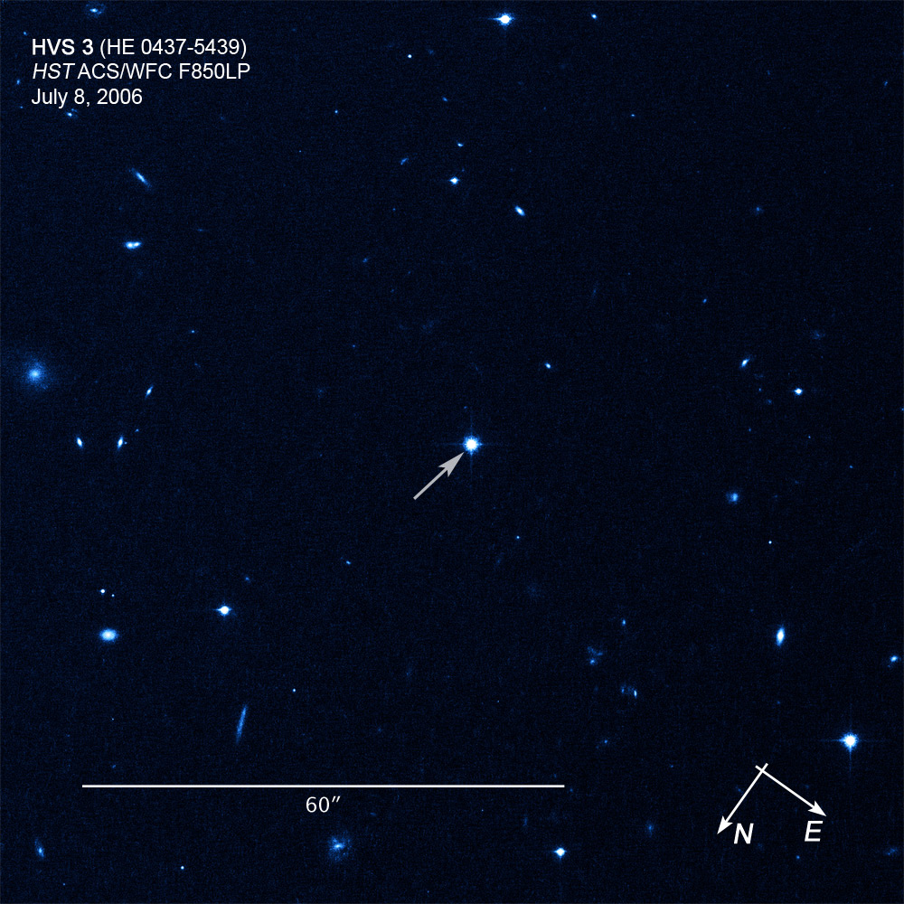
Astronomers have caught a number of hypervelocity stars zipping through the Milky Way since their first discovery in 2005. With speeds fast enough to escape the galaxy, hypervelocity stars were launched off course by some strong dynamical interaction. One such method, known as the Hills mechanism, predicts that when a binary star system approaches the Milky Way’s central supermassive black hole, one binary member is captured by the black hole and the other is flung away with high velocity.

However, constraining a hypervelocity star’s origin to the galactic center is limited by uncertainties in distances and proper motions, muddling how well researchers have been able to trace their orbits backward. Among a number of candidate galactic center–origin hypervelocity stars, only one has been confidently identified as having been kicked from the galaxy’s center. Intriguingly, this hypervelocity star and most galactic center–origin candidates are young, massive stars — old, low-mass hypervelocity stars from the galactic center have yet to be identified.

What does this dearth of old, low-mass zooming stars mean? Either stars in the galactic center are preferentially young and massive, with fewer than expected old and small stars, or low-mass hypervelocity stars are missed by selection effects, challenging to detect in current surveys. Searching for hypervelocity stars with higher precision and sensitivity may allow astronomers to tease out this missing population and trace back more zooming stars to a Hills mechanism origin.

Discovering An Old Hypervelocity Star

Leveraging high-quality spectra from the Dark Energy Spectroscopic Instrument (DESI) survey and precise astrometry from Gaia, Shunhong Deng (University of Chinese Academy of Sciences; China West Normal University) and collaborators reported the discovery of the hypervelocity star DESI-HVS1. From the spectroscopic and astrometric analyses, the authors determined that DESI-HSV1 is a ~14-billion-year-old low-metallicity star with a mass about 80% that of the Sun’s, moving through the galaxy at 523 km/s.
Backward orbit integration

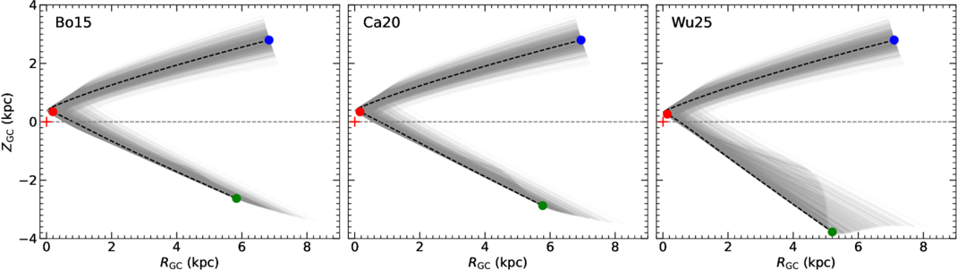
Backward-integrated orbits of DESI-HVS1 for three different galactic potential models. The blue, red, and green points show the star’s current position, closest approach to the galactic center, and position 50 million years ago, respectively. Click to enlarge. [Deng et al 2026]

Exploring the possible origins of this hypervelocity star, the authors integrated the star’s orbit backward in time for one billion years. The backward orbit integrations show the star approaching the galactic center where it then turns around, traveling away faster than the local escape velocity of the galaxy. Even when varying the galactic potential and constants, all orbit integrations suggest DESI-HVS1’s motion through the galaxy is most naturally explained by the Hills mechanism.

While more refined galaxy models and comparison to other candidate galactic center–origin hypervelocity stars are necessary to fully confirm its origins, DESI-HVS1 provides the first compelling evidence for an old, low-mass hypervelocity star candidate consistent with a galactic center launch. This suggests that the observed lack of such stars is likely not a reflection of the Milky Way’s central stellar population, but rather a consequence of observational constraints making such small hypervelocity stars particularly difficult to detect. As large spectroscopic and astrometric surveys continue to advance, the sample of galactic-center hypervelocity star candidates will grow, enabling further exploration of the stellar environment and dynamical processes at the Milky Way’s core.

Citation

“An Old, Low-mass, Metal-poor Hypervelocity Star Candidate Consistent with Galactic Center Origin,” Shunhong Deng et al 2026 ApJL 1003 L9. doi:10.3847/2041-8213/ae6505

The post Shot from the Heart of the Milky Way: Discovery of an Old Hypervelocity Star appeared first on AAS Nova.

NASA’s CloudCube Pioneers Miniaturized Radar to Study Clouds, Precipitation

10 June 2026 at 13:00

A compact, multifrequency radar built by a team at NASA’s Jet Propulsion Laboratory will make it easier to collect information about dynamic cloud systems. Called CloudCube, this new instrument simultaneously probes the atmosphere with three radar signals, spanning 36 to 240 GHz, for optimized sensitivity to a wide range of water droplet and ice particle sizes. 

An outdoor scientific equipment setup on a gravel surface under a bright blue sky. The main structure is a white shipping container elevated on concrete blocks, with a large, white, drum-shaped dome mounted on its roof. Attached to the front of the container is a grey metal cabinet featuring the red Jet Propulsion Laboratory (JPL) logo and a small angled panel on top. Bright green tie-down straps anchor the front equipment securely to the ground. Another container with a metal ladder is partially visible on the left.
Figure 1: A prototype of CloudCube’s G-band channel was installed at Cape Grim, Tasmania, as a guest instrument for the Department of Energy’s Cloud and Precipitation Experiment at Kennaook (CAPE-K)
Credit: Raquel Rodriguez Monje / JPL

Built with funding from NASA’s Earth Science Technology Office Instrument Incubator Program, CloudCube transmits and receives Ka-, W-, and G-band signals, making it the first compact radar system capable of simultaneously probing meteorological targets at wavelengths spanning approximately one to ten millimeters. Researchers will be able to combine information from the three signals to learn more about the initiation and evolution of precipitation, as well as cloud microphysics and radiative properties.

“We’re making a low-power, low-mass instrument to facilitate new cost-efficient missions for atmospheric observations. Building a multi-frequency radar, especially at G-band, is very novel,” said Raquel Rodriguez Monje, a systems engineer at JPL and principal investigator for CloudCube.

Each of CloudCube’s three signals observes a different element of cloud physics. Ka-band radar signals are ideal for collecting precipitation profiles; W-band radar signals are preferred for measuring cloud particles that give rise to precipitation; and G-band radar signals, which have never been collected from a space-based instrument, are ideal for measuring ice and liquid water content inside very light clouds (a paper describing this measurement can be found here).

Probing the atmosphere simultaneously with three signals allows researchers to collect data on all these cloud features at once, which is valuable for improving weather forecasts and especially climate modeling. CloudCube leverages innovations in millimeter-wave hardware to pack three radar modules–one for each signal–within a single compact system.

A highly intricate piece of custom electronic, likely radio frequency or microwave, hardware sitting on a light blue surface. The assembly is made mostly of thick gold-plated and silver metal blocks fastened together with numerous screws. It features several curved, rigid gold waveguides with flanged connections, various coaxial ports, a multi-pin D-sub connector, and a small bundle of colored electrical wires. A silver block on top is labeled with
Figure 2. A photo of the radar electronics for CloudCube’s compact G-band radar. Producing G-band radar signals requires a large amount of energy, and CloudCube is one of the first instruments to produce those signals effectively from a compact platform.
Credit: Raquel Rodriguez Monje / NASA JPL

One CloudCube innovation concerns the specialized components required to transmit G-band power from a compact, low-power instrument. The detection of cloud signals requires high transmit power, which CloudCube achieves by combining the outputs of multiple high-efficiency frequency-multiplication devices that allow the instrument to generate hundreds of milliWatts at 240 GHz. Another innovation of CloudCube is that it was designed to use as few radio frequency components as possible to reduce its mass and power consumption, which could lower the cost of future Earth-observing orbital instruments.

Flying an instrument equipped with G-band radar in space will be a new capability and will allow researchers to achieve greater spatial resolution and sensitivity in the study of cloud microphysical processes.

“Basically, we’re weighing clouds using these combinations of frequencies in a way that we couldn’t do before we had the G-band,” said Matt Lebsock, a researcher at JPL and co-investigator for CloudCube.

The instrument has been tested in the field. A ground-based prototype of CloudCube’s G-band channel operated continuously for 11 months during the Department of Energy’s Cloud and Precipitation Experiment at Kennaook (CAPE-K) campaign. CloudCube also participated in the Eastern Pacific Cloud Aerosol Precipitation Experiment, a ground campaign sponsored by the Department of Energy. A paper describing the results of that experiment can be found here.

Most recently, CloudCube successfully operated all three frequency bands from NASA’s Gulfstream III aircraft and collected its first airborne observations of snowfall as part of the North American Upstream Feature-Resolving and Tropopause Uncertainty Reconnaissance Experiment campaign—a NASA-funded campaign designed to improve forecasts of high-impact winter weather. The CloudCube team is currently calibrating and processing the data for public release.

For additional details, see the entry for this project on NASA TechPort.

Project Lead: Dr. Raquel Rodriguez Monje, NASA’s Jet Propulsion Laboratory

Sponsoring Organization: NASA’s Earth Science Technology Office Instrument Incubation Program

NASA’s CloudCube Pioneers Miniaturized Radar to Study Clouds, Precipitation

10 June 2026 at 13:00

A compact, multifrequency radar built by a team at NASA’s Jet Propulsion Laboratory will make it easier to collect information about dynamic cloud systems. Called CloudCube, this new instrument simultaneously probes the atmosphere with three radar signals, spanning 36 to 240 GHz, for optimized sensitivity to a wide range of water droplet and ice particle sizes. 

An outdoor scientific equipment setup on a gravel surface under a bright blue sky. The main structure is a white shipping container elevated on concrete blocks, with a large, white, drum-shaped dome mounted on its roof. Attached to the front of the container is a grey metal cabinet featuring the red Jet Propulsion Laboratory (JPL) logo and a small angled panel on top. Bright green tie-down straps anchor the front equipment securely to the ground. Another container with a metal ladder is partially visible on the left.
Figure 1: A prototype of CloudCube’s G-band channel was installed at Cape Grim, Tasmania, as a guest instrument for the Department of Energy’s Cloud and Precipitation Experiment at Kennaook (CAPE-K)
Credit: Raquel Rodriguez Monje / JPL

Built with funding from NASA’s Earth Science Technology Office Instrument Incubator Program, CloudCube transmits and receives Ka-, W-, and G-band signals, making it the first compact radar system capable of simultaneously probing meteorological targets at wavelengths spanning approximately one to ten millimeters. Researchers will be able to combine information from the three signals to learn more about the initiation and evolution of precipitation, as well as cloud microphysics and radiative properties.

“We’re making a low-power, low-mass instrument to facilitate new cost-efficient missions for atmospheric observations. Building a multi-frequency radar, especially at G-band, is very novel,” said Raquel Rodriguez Monje, a systems engineer at JPL and principal investigator for CloudCube.

Each of CloudCube’s three signals observes a different element of cloud physics. Ka-band radar signals are ideal for collecting precipitation profiles; W-band radar signals are preferred for measuring cloud particles that give rise to precipitation; and G-band radar signals, which have never been collected from a space-based instrument, are ideal for measuring ice and liquid water content inside very light clouds (a paper describing this measurement can be found here).

Probing the atmosphere simultaneously with three signals allows researchers to collect data on all these cloud features at once, which is valuable for improving weather forecasts and especially climate modeling. CloudCube leverages innovations in millimeter-wave hardware to pack three radar modules–one for each signal–within a single compact system.

A highly intricate piece of custom electronic, likely radio frequency or microwave, hardware sitting on a light blue surface. The assembly is made mostly of thick gold-plated and silver metal blocks fastened together with numerous screws. It features several curved, rigid gold waveguides with flanged connections, various coaxial ports, a multi-pin D-sub connector, and a small bundle of colored electrical wires. A silver block on top is labeled with "I" and "Q". A US quarter coin sits in the lower-left corner to indicate the scale of the device.
Figure 2. A photo of the radar electronics for CloudCube’s compact G-band radar. Producing G-band radar signals requires a large amount of energy, and CloudCube is one of the first instruments to produce those signals effectively from a compact platform.
Credit: Raquel Rodriguez Monje / NASA JPL

One CloudCube innovation concerns the specialized components required to transmit G-band power from a compact, low-power instrument. The detection of cloud signals requires high transmit power, which CloudCube achieves by combining the outputs of multiple high-efficiency frequency-multiplication devices that allow the instrument to generate hundreds of milliWatts at 240 GHz. Another innovation of CloudCube is that it was designed to use as few radio frequency components as possible to reduce its mass and power consumption, which could lower the cost of future Earth-observing orbital instruments.

Flying an instrument equipped with G-band radar in space will be a new capability and will allow researchers to achieve greater spatial resolution and sensitivity in the study of cloud microphysical processes.

“Basically, we’re weighing clouds using these combinations of frequencies in a way that we couldn’t do before we had the G-band,” said Matt Lebsock, a researcher at JPL and co-investigator for CloudCube.

The instrument has been tested in the field. A ground-based prototype of CloudCube’s G-band channel operated continuously for 11 months during the Department of Energy’s Cloud and Precipitation Experiment at Kennaook (CAPE-K) campaign. CloudCube also participated in the Eastern Pacific Cloud Aerosol Precipitation Experiment, a ground campaign sponsored by the Department of Energy. A paper describing the results of that experiment can be found here.

Most recently, CloudCube successfully operated all three frequency bands from NASA’s Gulfstream III aircraft and collected its first airborne observations of snowfall as part of the North American Upstream Feature-Resolving and Tropopause Uncertainty Reconnaissance Experiment campaign—a NASA-funded campaign designed to improve forecasts of high-impact winter weather. The CloudCube team is currently calibrating and processing the data for public release.

For additional details, see the entry for this project on NASA TechPort.

Project Lead: Dr. Raquel Rodriguez Monje, NASA’s Jet Propulsion Laboratory

Sponsoring Organization: NASA’s Earth Science Technology Office Instrument Incubation Program

The post NASA’s CloudCube Pioneers Miniaturized Radar to Study Clouds, Precipitation appeared first on NASA Science.

Could a White Dwarf–Black Hole Pair Explain the Longest Gamma-Ray Burst Ever Seen?

9 June 2026 at 23:36

illustration of GRB 250702B

What’s the story behind the longest gamma-ray burst ever observed? Researchers explore how repeated interactions between a white dwarf and an intermediate-mass black hole could explain GRB 250702B’s unusual properties.

An Exceptional Gamma-Ray Burst

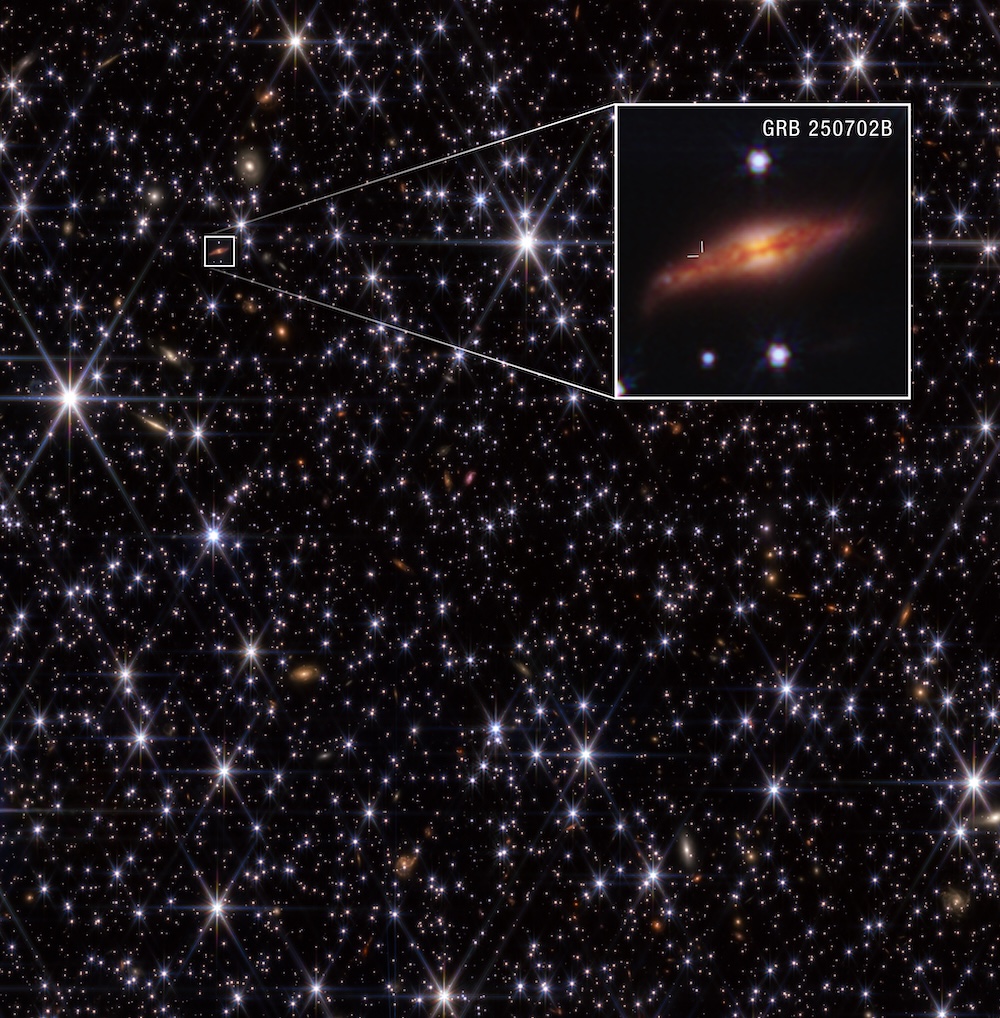
GRB 250702 host galaxy

An image of GRB 250702B’s location within its host galaxy. [NASA, ESA, CSA, H. Sears (Rutgers). Image Processing: A. Pagan (STScI)]

In 2025, the Fermi Gamma-ray Space Telescope spotted an intense flash of gamma rays from a distant, dusty galaxy, and a fleet of spacefaring and earthbound telescopes soon revealed the remarkable characteristics of the event. GRB 250702B featured multiple bursts spanning several hours, individual flares lasting roughly 100 seconds, and X-ray emission in the 24 hours leading up to the gamma-ray activity — something never seen before in a gamma-ray burst.

These characteristics have been challenging to explain with typical models of long gamma-ray burst formation, such as collapsing massive stars, but researchers have developed numerous promising alternatives. In a new research article, astronomers have shown how GRB 250702B’s behavior might be explained by repeated close encounters between a white dwarf and an intermediate-mass black hole.

Eccentric Close Encounters

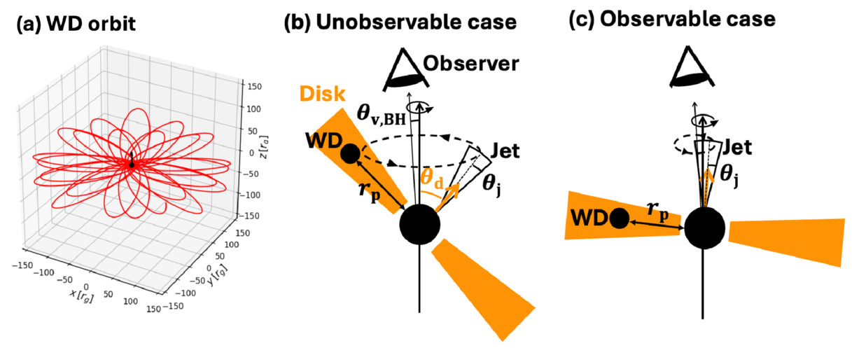
Yuri Sato (Tohoku University) and collaborators modeled the source of GRB 250702B as a white dwarf that has been captured into orbit around an intermediate-mass black hole. In their model, the white dwarf travels on an extremely eccentric orbit, drawing close to the black hole roughly once an hour. Each time the white dwarf ventures close, the black hole’s tidal forces strip away part of the star until, after about 40 such encounters, the white dwarf is completely destroyed.

geometry of the GRB 250702B system

Schematics showing the orbit of the white dwarf (WD; left) and the geometries that produce observable and unobservable jets. Click to enlarge. [Sato et al. 2026]

When the black hole peels material away from the white dwarf, some material swirls into an accretion disk, and some is cast off into space. Accretion from the disk powers a narrow relativistic jet: the source of the event’s powerful gamma-ray flares. This should mean that there is one jet produced each time the white dwarf is partially disrupted — 40 times — yet astronomers detected only a handful of flares from GRB 250702B.

Jet Precession and Model Predictions

The discrepancy can be resolved if the angle between the jet and the black hole’s spin axis precesses over time so that only some of the jets are pointed toward us. This can occur if the accretion disk is misaligned relative to the black hole’s spin. As an alternative, disk instabilities or other processes could keep all but a few of the expected jets from being launched.

radio afterglow predictions for GRB 250702B

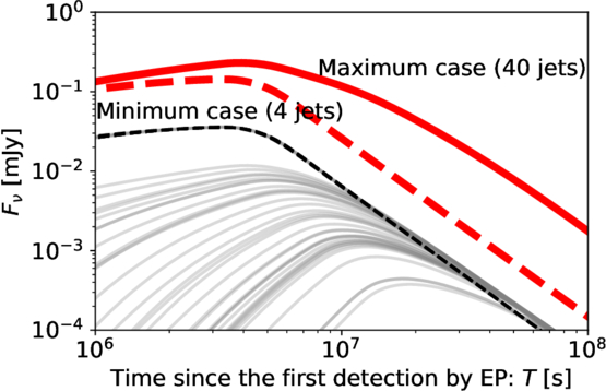
Predicted strength of the radio afterglow for the jet precession case (maximum case) and the case in which only four jets were launched due to disk instabilities or jet choking (minimum case). The x-axis shows the time since the burst was detected in X-rays by the Einstein Probe (EP). [Sato et al. 2026]

Sato and coauthors found that these two scenarios have different long-term outcomes, providing a potential way to ascertain what’s going on at the source; in the jet precession scenario, the jets that are launched away from our line of sight produce an order of magnitude more radio emission at late times.

This work by Sato and collaborators demonstrates how the repeated partial tidal disruption of a white dwarf by an intermediate-mass black hole can match the properties of one of the most remarkable recent transient sources — one that has pushed astronomers to consider new ways of producing gamma-ray bursts.

Citation

“Successive Partial Disruptions with Orbital Precession in a White Dwarf–Black Hole System for Repeating GRB 250702B,” Yuri Sato et al 2026 ApJL 1003 L44. doi:10.3847/2041-8213/ae6a8f

The post Could a White Dwarf–Black Hole Pair Explain the Longest Gamma-Ray Burst Ever Seen? appeared first on AAS Nova.
Shining a Light on the Shadowy Movements in Saturn’s Rings

8 June 2026 at 17:00

Editor’s Note: Astrobites is a graduate-student-run organization that digests astrophysical literature for undergraduate students. As part of the partnership between the AAS and astrobites, we occasionally repost astrobites content here at AAS Nova. We hope you enjoy this post from astrobites; the original can be viewed at astrobites.org.

Title: Dynamics of Planetary Rings Under Thermal Forces
Authors: Wen-Han Zhou et al.
First Author’s Institution: The University of Tokyo
Status: Published in ApJL

If you ask anyone what their favourite planet is, the answer you’ll most likely hear is Saturn. Why? Why else than the beautiful and intricate ring system surrounding the gas giant. The other gas and ice giants in our solar system — Jupiter, Uranus, and Neptune — have ring systems themselves but none quite as striking as Saturn’s. Would it surprise you to learn that astronomers’ best models have not yet totally explained why Saturn’s rings look the way they do?

In contrast, it may not surprise you to hear that people have been trying to explain the rings for as long as we have seen them with telescopes. We now know that planetary rings are collections of relatively small particles (think micrometre up to metre sized), most likely having once been the material of a larger body that was disrupted either by collisions or tidal forces. This material, due to the gravity of its local planet, is sculpted into a flat disc where more subtle interactions then lead to substructure forming within the disc such as gaps and ringlets. Many of these substructures are explained by well-understood physics — for example gaps being carved by embedded moonlets or resonances sculpting ring edges — though there remain some outstanding problems in our understanding.

The authors of today’s article set their sights on the problematic inner edge of Saturn’s A ring (Figure 1). They describe some mechanisms — namely the collisions of micrometeoroids within the rings — by which a sharp ring edge can be maintained, but there exists a gap in the understanding of how such an edge can form in the first place. All hope is not lost, though, as today’s authors reintroduce a physical process they call the “eclipse–Yarkovsky” effect, which seems to explain these phenomena.

horizontally sliced Saturn's rings

Figure 1: A horizontally sliced image of Saturn’s rings shows the rich substructure and gaps within the various rings. Saturn, which is not shown here, would be to the left of the image. The authors of today’s article are particularly concerned with the bright and sharp inner (left side) edges of the A and B rings. Click to enlarge. [NASA/JPL/Space Science Institute]

Billions of Rocket-Powered Bumper Cars

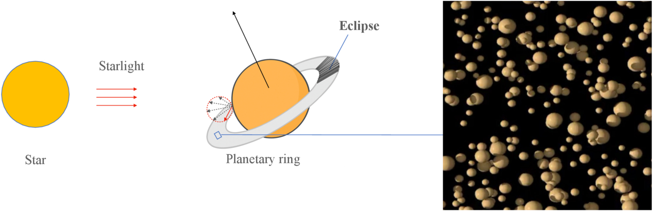
The idea behind this process revolves entirely around light. When sunlight hits a particle within a planetary ring, non-absorbed sunlight imparts a little “bump” onto a particle, ever so slightly altering its trajectory. At the same time, some of the sunlight is absorbed into the particle, which heats it up; light is soon re-emitted via thermal radiation, which, again, can slightly change the trajectory of these tiny particles. From a point on the surface of each ring particle (see rightmost side of Figure 2), the photons from this thermal radiation are all emitted in random directions; however, across the whole surface of the particle there is a net force! These tiny particles are spinning, and so the side just near “sunset” is hottest and emitting the most thermal photons. In this way, the pressure from the sunlight plus the thermal radiation of each particle imparts a net torque on the ring itself which changes the angular momentum of the ring.

diagram showing sunlight falling on Saturn and the planet casting a shadow on its rings

Figure 2: Starlight is the main source of light onto the particles that make up a planetary ring (right panel) though reflected light from the planet’s surface hits it too. This light “heats up” the ring and forms an asymmetry as the ring is eclipsed by the planet, which produces a net force. [Zhou et al. 2026]

What we described just then is essentially solar radiation pressure plus the Yarkovsky effect. It turns out that the net force from this process typically averages out to zero as the ring particles orbit around the planet. This assumes, though, that the sunlight is constantly shining on the ring. Stunning imagery of Saturn tells us that this isn’t the case, so what happens when we take into account the shadow cast on the ring from the planet? Today’s authors find that the net effect induces a positive change in angular momentum of the ring particles, which they call the eclipse–Yarkovsky effect.

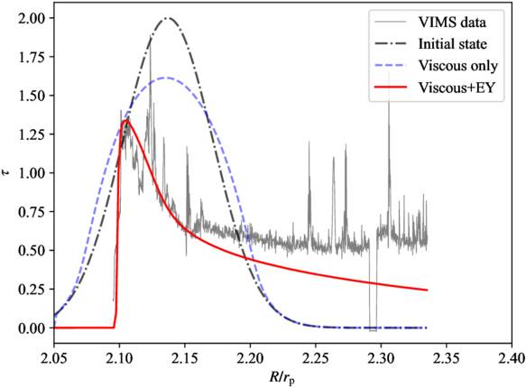
After today’s authors detailed all of the math involved in this process (and there is a lot), they put it into practice to try to help explain Saturn’s curious rings. Including the eclipse–Yarkovsky effect together with other known effects that drive ring evolution allowed them to reproduce the optical depth profile (how thick the ring looks) of Saturn’s A ring better than ever before (notably the sharp inner edge in Figure 3). On top of this, the effect provides another avenue for moonlet formation in the outer edges of ring systems as the positive torque from the effect drives material out toward and away from the Roche limit.

plot of optical thickness versus radius

Figure 3: The authors try to explain the current structure of Saturn’s A ring by initialising it with a Gaussian profile of optical thickness versus radius (black dot-dashed line) and evolving it for 81 million years under different effects. When viscous effects are included (blue dashed line), the ring spreads out, but it’s only when the eclipse–Yarkovsky (EY) effect is included (red line) that the model closely matches the observed data (grey line). [Zhou et al. 2026]

Undeniably useful for Saturn, the eclipse–Yarkovsky effect may also explain some other conundra in the solar system. Mars may have once had rings, which are thought to have eventually clumped together to form the inner moon Phobos. This idea is problematic, though, in that current models suggest there should still be some residual ring system around Mars even after Phobos formed. Enter the eclipse–Yarkovsky effect: being 100 times stronger for Mars than Saturn (due to its more intense incident sunlight), the effect may have driven out and dispersed that residual ring altogether. While the authors are currently looking into this possibility, the reintroduction of the eclipse–Yarkovsky effect has already shown great promise for our most beautiful ringed planetary neighbour.

Original astrobite edited by Wasi Naqvi.

About the author, Ryan White:

I am a first-year PhD student at Macquarie University in Australia, working mainly on binary/multiple systems with massive stars (Wolf–Rayets in particular!). Outside of study, I’m probably drinking coffee, baking, reading, or going for a run. You can also find me procrastinating on Bluesky @astroryan.bsky.social.

The post Shining a Light on the Shadowy Movements in Saturn’s Rings appeared first on AAS Nova.
Courtside Seats on Mars

5 June 2026 at 17:00

A photograph of an entire visible hemisphere of Mars.

When the third known object from the galactic space beyond our Sun barreled through the solar system last year, Earth was in a terrible spot to view its flyby. Thankfully, however, a spacecraft that was previously busy mapping Mars took advantage of much better positioning for a closer look.

Cheap Seats

Astronomers have now observed three interstellar objects as they’ve flown through the solar system: 1I/ʻOumuamua, which shocked astronomers in 2017; 2I/Borisov, which followed in 2019 and behaved almost identically to a solar system comet; and now 3I/ATLAS, which was found buzzing toward the Sun in July 2025. As soon as 3I/ATLAS was spotted, pretty much every telescope on the planet took a look. The data swiftly revealed much that intrigued astronomers: while 3I/ATLAS was behaving essentially like a standard comet, its chemistry was nothing like its solar system counterparts, and its coma and dust outflow were strangely shaped. Among other oddities, it seemed to counterintuitively have a dust tail that pointed toward the Sun.

A plot showing that Earth-based observations could only get as best a 20-degree out-of-plane view, while Mars-based observations could get up to nearly 40.

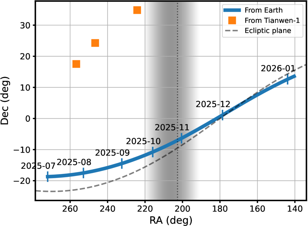
3I/ATLAS’s path across the sky as seen from Earth versus the clearer line of sight from Mars. The shaded region represents the times where the comet was too close to the Sun for viewing. [Xin Ren et al. 2026]

Unfortunately for astronomers, 3I/ATLAS didn’t make it easy for them to study the shape of its coma. Thanks to a cosmic coincidence, the interstellar visitor was traveling almost perfectly within the plane of our solar system, and Earthbound observers were often limited to an edge-on view of its tail. Even worse, 3I/ATLAS looped around the back of the Sun from our perspective, meaning no one on the planet could observe the comet for a few weeks in the fall. This led a group of astronomers to consider their assets that are farther from home.

Better View from Mars

The Tianwen-1 spacecraft, which entered Martian orbit in early 2021 and has been diligently mapping the Red Planet ever since, has a high-resolution camera that’s normally pointed at the planet’s surface. By spinning the spacecraft around, a team of researchers led by Xin Ren (National Astronomical Observatories, Chinese Academy of Sciences) repurposed the camera to act as a small telescope when 3I/ATLAS flew by. In another cosmic coincidence, 3I/ATLAS happened to pass very near Mars last fall, and this close approach gave Tianwen-1 a great out-of-plane view of the coma. The orbiter managed to capture 57 images of 3I/ATLAS over three days last fall, representing China’s first-ever observations of an object from an asset in deep space.

Multi-panel photographs of a comet against a background of streaked stars.

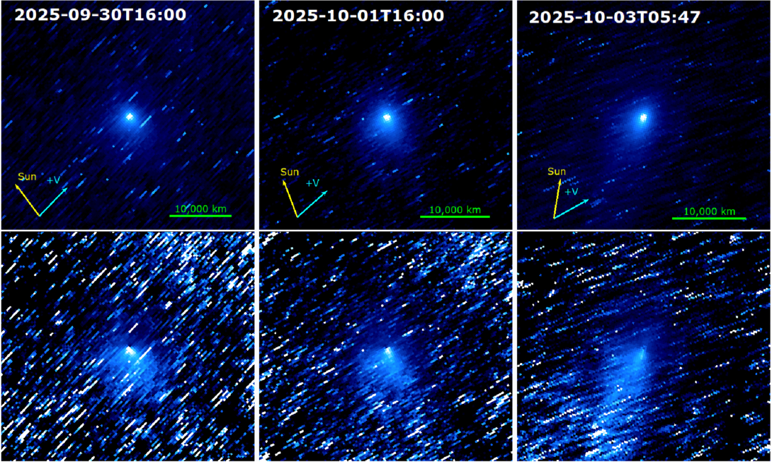
Stacked images of 3I/ATLAS from the Tianwen-1 orbiter across three epochs; the tail’s apparent shape shifts as the viewing geometry changes. Click to enlarge. [Xin Ren et al. 2026]

The team took full advantage of the great view and leveraged the spacecraft’s unique perspective to extract some intriguing results. By tracking how the gentle pressure of sunlight nudged the escaping grains, the researchers found that the coma is dominated by surprisingly large dust. With an average size of hundreds of microns across, the dust is more like coarse sand than smoke, and they found that it ambles away from the comet at just 3–10 meters per second. All told, 3I/ATLAS was shedding dust at roughly 1,000 kilograms every second. The big grains may be a fingerprint of a cold, distant birthplace: models suggest such grains collect in the frigid outer reaches of planet-forming disks, hinting that 3I/ATLAS was forged far from its parent star before being flung into the dark.

As new surveys begin to turn up interstellar interlopers more often, this improvised observation makes a tidy point: the spacecraft already scattered across the solar system can double as a fleet of opportunistic comet-watchers, each offering a view we simply can’t get from home.

Citation

“Interstellar Object 3I/ATLAS Observed from Mars by China’s Tianwen-1 Spacecraft,” Xin Ren et al 2026 ApJL 1003 L10. doi:10.3847/2041-8213/ae61b3

The post Courtside Seats on Mars appeared first on AAS Nova.
Now That’s Metal: How to Spot Stars That Have Swallowed Their Planets

3 June 2026 at 17:00

An illustration of an exoplanet about to be engulfed by its host star

Planets that get too close to their host stars are liable to be engulfed and consumed. New research explores how to identify stars that have had a planetary snack.

It’s Snack Time

Being a planet that closely orbits its star is dangerous, and various dynamical processes can draw a planet inward past the point of no return. When a planet vanishes beneath the surface of its host, it eventually disintegrates within the star, its atoms mixing into the blazing stellar soup.

This outcome is likely extremely common across the universe, and researchers have begun to see evidence for it: stars that appear to have absorbed angular momentum from their planets, white dwarfs with uncanny metals in their spectra, and stars with chemical abundances that don’t match those of their siblings. Now, in a recent publication led by Kaitlyn Lane (Vanderbilt University), researchers seek to find observational signatures of planetary engulfment of rocky exoplanets by main-sequence stars.

Modeling Engulfment

Lane’s team focused on main-sequence stars in the range of 0.5 to 1.4 solar masses, using one-dimensional analytical models to determine which of these stars will most readily display signs of having engulfed a planet. They simulated the stars as they consumed either an Earth-like planet or a super-Earth with the same composition as Earth but 15 times its mass.

illustration of a planet being engulfed by its star

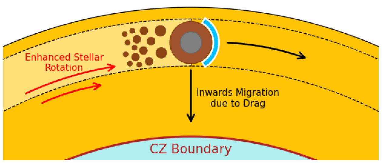
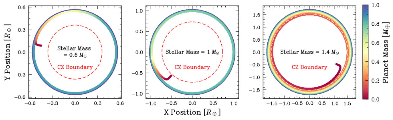
Diagram showing a planet being engulfed by its star and beginning to disintegrate before migrating inward. The boundary between the star’s outer convective zone (CZ) and inner radiative zone is shown. Click to enlarge. [Lane et al. 2026]

At the onset of the model, the engulfment is set to begin, the planet placed tangent to the star’s surface. The planets sink down and orbit just barely within their stars for 1–10 years, their solid surfaces slowly beginning to evaporate.

After that relatively lengthy phase, the process proceeds rapidly: as the planet inches deeper into its star, the drag forces grow stronger and the planet’s demise accelerates, with the planet disintegrating over the course of hours. In the last phase, the planet makes its final plunge and is destroyed in a half hour.

Signs of Planets Past

Lane’s team found that the planets tended to be destroyed fully within the outer convective layer of their stars, except in the case of the most massive stars studied here. For more massive stars, the outer convective zone is shallower than it is for the less massive stars, allowing a chunk of each planet to survive the passage through the convective zone to reach the radiative zone below.

simulation results showing planets disintegrating within their host stars

The trajectories of three example cases, showing how the planet loses mass as it spirals inward. In the 1.4-solar-mass case, part of the planet survives to reach the radiative zone, but the shallowness of the star’s convective zone means that the disintegrated planetary material is easier to observe. Click to enlarge. [Lane et al. 2026]

What this translates to, for the purposes of identifying planet-eating stars from afar, is that stars near the top of the mass range studied — from 1.0 to 1.4 solar masses — make the best targets. This is because the tell-tale planetary metals are not overly diluted within the stars’ relatively small convective zones, making these elements easier to detect. In terms of specific metals, the authors found that aluminum, calcium, and vanadium are the best signposts of planetary engulfment, with lithium also making the list.

While the authors acknowledge that there’s more work to be done — they plan to investigate the impacts of planetary engulfment on stellar structure more closely, for example — this work represents an important foray into identifying targets for future studies of stars that have eaten their planets.

Citation

“Observable Metal Pollution in Main-Sequence Stars: Simulations of Rocky Planets Engulfed by Stars in the 0.5 to 1.4 M⊙ Range,” Kaitlyn T. Lane et al 2026 ApJ 1003 67. doi:10.3847/1538-4357/ae5b9a

The post Now That’s Metal: How to Spot Stars That Have Swallowed Their Planets appeared first on AAS Nova.
The First Starspot Spectrum Revealed by JWST

2 June 2026 at 17:00

M-dwarf star with starspots

Editor’s Note: Astrobites is a graduate-student-run organization that digests astrophysical literature for undergraduate students. As part of the partnership between the AAS and astrobites, we occasionally repost astrobites content here at AAS Nova. We hope you enjoy this post from astrobites; the original can be viewed at astrobites.org.

Title: A Panchromatic JWST Spectrum of a Giant Starspot on the Fully Convective M Dwarf TOI-3884
Authors: C. A. Murray et al.
First Author’s Institution: University of Colorado Boulder
Status: Published in ApJ

We often picture stars as smooth, glowing spheres, as if they’ve been run through an Instagram filter. But real stars have spots: cooler, darker regions on a star’s surface caused by strong magnetic fields.

Annoyingly, these spots can seriously interfere with how we study exoplanet atmospheres.

How to Probe a Planetary Atmosphere

Planetary atmospheres are often probed through transmission spectroscopy. When a planet transits its star, some starlight passes through the planet’s atmosphere before reaching us. We can distinguish the light that has passed through the planet’s atmosphere by comparing the star’s light in transit versus out of transit. In doing so, we can isolate the atmospheric spectrum and look for absorption features of species like water or oxygen.

Easy, right?

How Starspots Get in the Way

Things get more complicated once we stop thinking of the star as if it’s been smoothed out by an Instagram filter. Starspots are cooler than the surrounding stellar surface, which means they emit a different spectrum. They are also constantly changing: new spots can form, old ones can disappear, and the star’s rotation carries them in and out of view. This changes things.

First of all, your star’s spectrum changes over time, which could mean that the star’s spectrum out of transit is not the same as the star’s spectrum during transit. On the other hand, the planet may transit across a starspot instead of a “normal” stellar region. In this case, the light we measure during the transit is affected by the spot, and it is no longer accurate to directly compare it with the overall stellar light outside the transit.

Ultimately, absorption features that we thought were from the planetary atmosphere could actually be coming from starspot contamination instead.

Starspot Models: Our Solution?

To deal with this, astronomers build starspot models, where they vary the spots in terms of the following:

  • The surface covering fraction: this parameter tells us how much of the stellar surface is covered in spots
  • The temperature contrast: this parameter tells us how much cooler (in ratio) the spot is compared to the rest of the stellar surface, and by proxy how much dimmer

These models are promising, but how do we know that we have chosen the right parameters?

A Unique Laboratory: TOI-3884

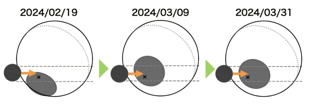
The TOI-3884 system is a unique laboratory for testing our starspot models. As seen in Figure 1, it has very convenient starspot geometry, with a large starspot located close to its pole. On top of that, we observe this star almost completely pole-on, which means that we always see this starspot, no matter how much the star rotates. To top this all off, the star hosts a close-in planet, which orbits the star from pole to pole.

Illustration of the TOI-3884 system

Figure 1: Illustration of the TOI-3884 system. The pole (and rotation axis) of the star is indicated with a black “x,” indicating that we see the star almost pole-on. The polar starspot is indicated in grey, and the transiting planet TOI-3884b is indicated in black. Different dates are shown, illustrating how the system evolves over the span of a few weeks. [Adapted from Mori et al. 2025]

The planet transits the star, and as it does so, it always passes over the polar starspot. This gives us a rare opportunity to probe the spectrum of a starspot. Similar to how we can use normal in/out of transit observations to probe a planetary atmosphere, we can now compare the observations during/after a “starspot transit” to probe the starspot region. Today’s authors do exactly this using six different transit observations from JWST.

So… How Good Are Our Models?

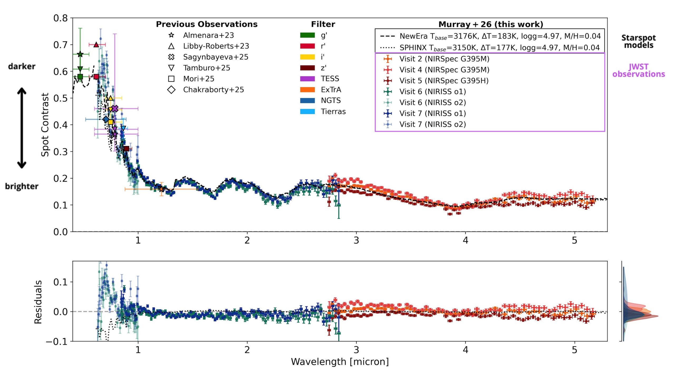
From the JWST observations, the authors extract a starspot spectrum for the first time. Figure 2 shows this as the spot contrast (how much dimmer the spot is than the surrounding stellar surface) plotted across different wavelengths. To see how well our models are doing, they compare this observed spectrum to two commonly used starspot models. The difference between the data and the models (the residual) is plotted in the lower panel.

spectrum of TOI-3884’s starspot.

Figure 2: The spectrum of TOI-3884’s starspot. The y-axis in the upper panel, the spot contrast, indicates how much dimmer the starspot is compared to the “normal” stellar surface. Different observations taken with JWST are indicated in different colored crosses, and other previous observations are overplotted in various other shapes. Model starspot spectra are shown in dashed or dotted black lines. The residuals between the model spectra and the JWST observations are shown in the bottom panel. [Adapted from Murray et al. 2026]

At wavelengths longer than about 1 micron, in the near-infrared regime, things look good! The residuals stay small, meaning the models do a solid job reproducing the observations. But move left into shorter wavelengths, in the optical regime, and the agreement quickly falls apart. The residuals grow, and it becomes clear that the models are missing something.

There’s still work to be done before we can confidently probe planetary atmospheres at optical wavelengths without worrying about stellar contamination, and this observed starspot spectrum provides a unique benchmark to test future starspot models. For now, the near-infrared remains a safer and more reliable window for planet atmosphere studies.

Original astrobite edited by Natalie Price.

About the author, Elise Koo:

I’m a PhD student at the University of Amsterdam, working to detect magnetic interactions between stars and their planets using radio and spectroscopic observations. Outside of research, I like to try out a variety of sports.

The post The First Starspot Spectrum Revealed by JWST appeared first on AAS Nova.
Featured Image: Massive Young Star Clusters, Revealed

1 June 2026 at 17:00

The Antennae galaxies are a nearby pair of interacting galaxies, shown in optical light from the Hubble Space Telescope (left) and in infrared light from JWST (right) in the image above. Between the two galaxies’ bright nuclei, there is a vast and dusty molecular cloud complex that harbors a large number of massive young star clusters — and in a recent article led by Rupali Chandar (University of Toledo), researchers have worked to pin down exactly how many clusters are embedded within the dusty whorls of the Antennae galaxies. The team used JWST to search for emission from star clusters too thickly blanketed with dust to be visible in previous observations by Hubble. They ultimately identified 45 sources, 40 of which were seen for the first time in this study. These star clusters mostly inhabit the overlap region between the two galaxies, are less than 2.5 million years old, and each contain roughly 104–106 solar masses. To learn more about how JWST’s infrared capabilities unveiled young star clusters in these interacting galaxies, be sure to check out the full article linked below.

Citation

“Nowhere Left to Hide: Uncovering All of the Massive Young Embedded Star Clusters in the Antennae with JWST,” Rupali Chandar et al 2026 ApJ 1002 64. doi:10.3847/1538-4357/ae56e8

The post Featured Image: Massive Young Star Clusters, Revealed appeared first on AAS Nova.
Stacking Up the Discovery of Six Millisecond Pulsars

29 May 2026 at 17:00

Millisecond pulsar and companion artist's impression

The fastest spinning pulsars in the universe are often quite difficult to detect. Leveraging multiple observations from the largest single-dish telescope in the world, researchers have discovered six previously undetected pulsars.

Millisecond Pulsars in Globular Clusters

Globular clusters, compact collections of tens of thousands to millions of stars, are highly dense and rife with dynamical interactions. These active environments are ideal factories for the formation of millisecond pulsars — the extremely fast-spinning cores of once-massive stars, shining beams of radio emission from their poles. One way millisecond pulsars are thought to form is when a pulsar in a binary system steals mass from its companion star, transferring angular momentum and causing the pulsar to spin up. The densely packed environment in a globular cluster provides ample opportunity for a pulsar to acquire a companion to siphon.

However, millisecond pulsars in distant globular clusters are notoriously difficult to detect. Traditional pulsar searches that rely on a single observation tend to miss millisecond pulsars, many of which have signals too faint to be distinguished from noise or radio interference. Instead, researchers must rely on a different method to find these fast-spinning pulsars.

FAST

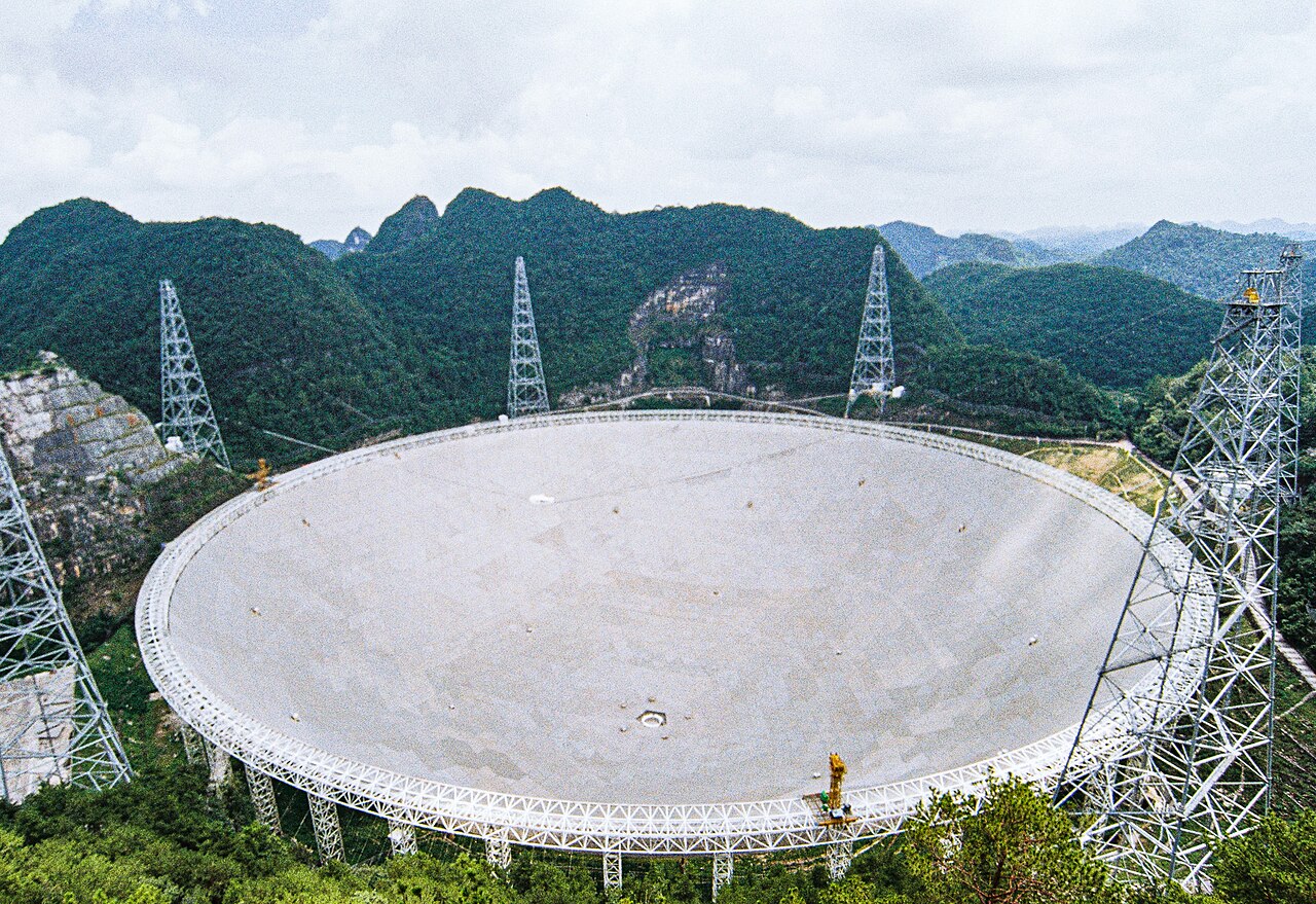
FAST, the 500-meter single-dish radio telescope located in southwestern China. [Wikipedia user SCJiang; CC BY 4.0]

Stack Search Success

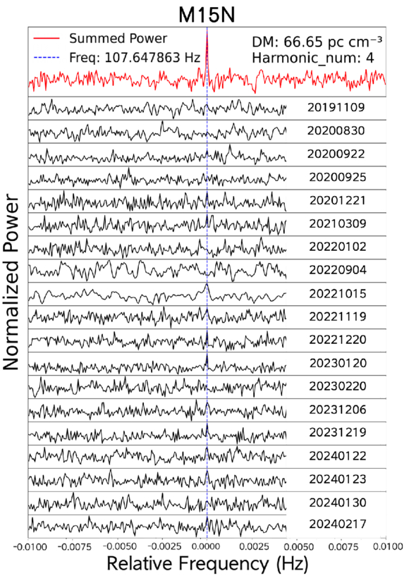
To find faint millisecond pulsars, researchers have developed the stack search method, in which multiple radio observations are combined to tease out faint signals and decrease noise. Reliably stacking observations across epochs requires stability; isolated millisecond pulsars, now no longer spinning up after losing their companion, have very stable rotation periods, making them ideal targets for the stack search method. To date, the stack search method has successfully identified nine isolated globular cluster millisecond pulsars using data from the Arecibo, Parkes, and Green Bank radio telescopes.

Stack Spectra

Power spectra from a discovered millisecond pulsar M15N. The black solid lines show the 19 individual observations of the pulsar, and the red solid line in the top panel shows the stacked spectrum. The stack search method pulls out a clear pulsar signal. [Dai et al. 2026]

In hopes of recovering more of these faint fast-spinning pulsars, Yinfeng Dai (Beijing Normal University) and collaborators used archival data obtained with the Five-hundred-meter Aperture Spherical radio Telescope (FAST), the world’s largest single-dish telescope. Targeting two specific globular clusters, NGC 6517 and M15, the team applied the stack search method to 23 and 19 observations of the globular clusters, respectively. From their search, the authors discovered six previously unidentified isolated millisecond pulsars: four in NGC 6517 and two in M15.

While previous studies identified brighter pulsars in the targeted globular clusters, the authors confirmed that all six newly discovered pulsars are too weak to be reliably recovered from single-epoch searches, underscoring the importance of the stack search method. In particular, this search increased the known pulsar populations of NGC 6517 and M15 by 27% and 18%, respectively, suggesting that a meaningful fraction of globular cluster pulsars are easily missed in traditional pulsar searches. Future studies employing this stack search method will continue to detect faint millisecond pulsars, unlocking this elusive population for further exploration.

Citation

“The Stack Search Tests on FAST Data: Discovery of Six Faint Isolated Millisecond Pulsars in NGC 6517 and NGC 7078 (M15),” Yinfeng Dai et al 2026 ApJL 1002 L31. doi:10.3847/2041-8213/ae5dbb

The post Stacking Up the Discovery of Six Millisecond Pulsars appeared first on AAS Nova.
Third Star’s the Charm: Most Merging Black Holes Might Be in Triple Systems

27 May 2026 at 17:00

Illustration of merging black holes

Where do black hole mergers happen? Recent research finds evidence that most black hole mergers occur in triple systems containing a close inner binary and a more distant third party.

Assembling Merging Black Holes

Thanks to the combined efforts of the LIGO, Virgo, and KAGRA gravitational wave detectors, we’ve now collected the subtle signals from several hundred pairs of merging stellar-mass black holes. As this collection of spacetime ripples continues to grow, researchers are seeking to understand how these merging black hole pairs were assembled.

In the simplest scenario, pairs of high-mass stars independently evolve into black holes, lose momentum by emitting gravitational waves, and meld into one another. But the population of merging black holes likely contains contributions from multiple sources, including multiple-star systems, the disks surrounding accreting supermassive black holes, and black holes that have already experienced a merger. Which of these merging populations is reflected in our catalog of gravitational wave events?

Modeling Challenges

spin–orbit tilt diagram

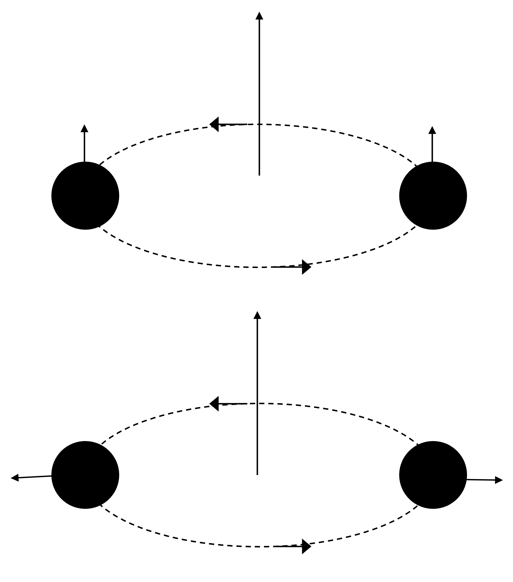
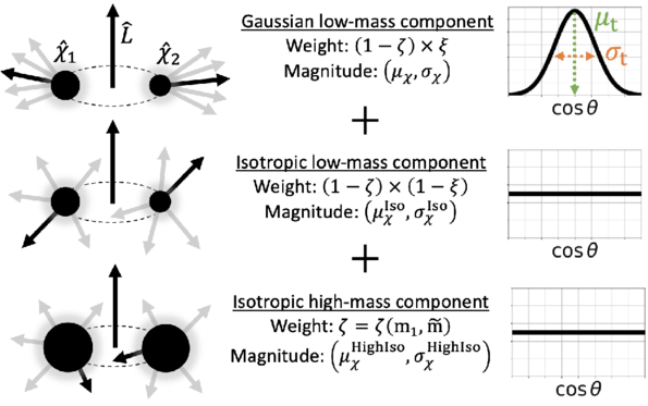
A black hole binary system with aligned spins and orbit (top) and a binary with spins tilted by 90 degrees (bottom). [AAS Nova/Kerry Hensley]

In theory, this question can be answered by extracting the properties of merging black holes — mass, spin, and the like — from gravitational wave observations and comparing these properties against model predictions from different formation pathways. In reality, this is exceedingly difficult, as certain merger pathways can produce a wide variety of results, depending on assumptions or fine tuning.

So far, the increasingly large pool of gravitational wave detections tentatively points to a feature that could illuminate the sites of black hole mergers: a peak in the spin–orbit tilt distribution around 90 degrees. This feature has been most confidently extracted from nonparametric analyses, which do not make assumptions about the population of merging black holes, but it has also been hinted at in parametric analyses, which do make population-level assumptions.

Triple-System Feature

To investigate this feature further, a team led by Jakob Stegmann (Max Planck Institute for Astrophysics) performed a new, astrophysically motivated parametric analysis of the most recent catalog of gravitational wave detections from LIGO, Virgo, and KAGRA.

black hole populations used in modeling the observed spin–orbit tilt distribution

The three populations in the team’s modeling. [Stegmann et al. 2026]

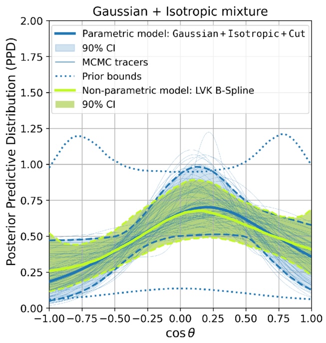
Their modeling tests combinations of multiple populations, including mergers in isolated binary systems, triple-star systems, and dense environments like star clusters. They also include a potential contribution from higher-mass mergers involving black holes that have merged previously. Using this framework, Stegmann’s team found that the observed spin–orbit tilt distribution is best matched by a model dominated by mergers in triple-star systems, with some contribution from other sources.
Posterior predictive distribution of black hole spin–orbit tilts

Posterior predictive distribution of black hole spin–orbit tilts. Both the authors’ modeling (solid blue line) and the nonparametric modeling performed by the LIGO–Virgo–KAGRA collaboration (solid green line) find evidence for a peak in the spin–orbit tilt distribution near cosθ = 0. [Adapted from Stegmann et al. 2026]

Specifically, this finding suggests that most mergers occur in hierarchical triple systems, which naturally predict an excess of 90-degree spin–orbit tilts without any fine tuning. Hierarchical triples contain an inner close binary with a distant outer companion; in these systems, relativistic spin precession, gravitational wave emission, and oscillations in eccentricity and inclination work to tilt the black holes in the inner binary by 90 degrees.

Stegmann and collaborators pointed out that the triple-system scenario aligns well with other properties of the observed population of black hole mergers, such as the mass and effective spin distributions. This scenario may also be necessary to explain certain merging pairs that might have had slightly eccentric orbits at the moment of merging. If future gravitational wave observations strengthen the evidence for a peak in the spin–orbit tilt distribution near 90 degrees, it will have profound implications for how and where black holes merge in our universe.

Citation

“Gravitational-Wave Observations Suggest Most Black Hole Mergers Form in Triples,” Jakob Stegmann et al 2026 ApJL 1000 L59. doi:10.3847/2041-8213/ae52ec

The post Third Star’s the Charm: Most Merging Black Holes Might Be in Triple Systems appeared first on AAS Nova.
Life on the (Red) Edge

26 May 2026 at 17:00

Earth in visible and near-infrared light

Editor’s Note: Astrobites is a graduate-student-run organization that digests astrophysical literature for undergraduate students. As part of the partnership between the AAS and astrobites, we occasionally repost astrobites content here at AAS Nova. We hope you enjoy this post from astrobites; the original can be viewed at astrobites.org.

Title: Retrieving the Red Edge on Earth-Like Planets with Heterogeneous Clouds and Surfaces
Authors: Zachary Burr et al.
First Author’s Institution: Jet Propulsion Laboratory; ETH Zurich
Status: Published in ApJ

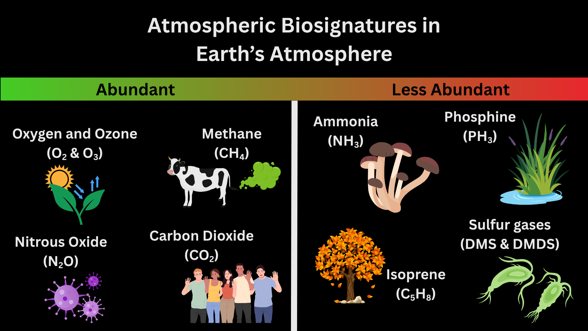
In the next 25 years, astronomers could find signs of life on other planets with the launch of the Habitable Worlds Observatory. Atmospheric signs of life, known as atmospheric biosignatures, are how astronomers currently search for life on other planets. Figure 1 shows examples of atmospheric biosignatures with pictures of each chemical’s origin on Earth. Before E.T. can phone home, though, we have to understand what chemicals make up a planet’s atmosphere. To do this, astronomers can use spectroscopy to observe a planet’s atmosphere in different wavelengths and measure the types and quantities of chemicals present.

biosignatures in Earth's atmosphere

Figure 1: Atmospheric biosignatures present in Earth’s atmosphere. More abundant biosignatures include oxygen and ozone (byproducts of photosynthesis in plants and bacteria) and nitrous oxide (byproduct of bacteria that don’t need oxygen to survive). Less abundant biosignatures include isoprene (released from the breakdown of leaves that have fallen from trees) and sulfur gases (byproducts of cyanobacteria). [Kaz Gary]

There are many ways to observe the spectrum of a planet, but the one you’re probably most familiar with is transmission spectroscopy. You can learn more about transmission spectroscopy of exoplanet atmospheres and how to model transmission spectra with these bites: 1, 2, 3. However, all of the current techniques for exoplanet spectroscopy (including transmission spectroscopy) measure the star’s light and how the planet affects the star’s light. This means it’s heavily dependent on how we model the star’s light to indirectly observe the planet’s light. The only way to take the spectrum of a planet directly is with direct imaging: the technique that the future Habitable Worlds Observatory will use to find signs of life in planetary spectra.

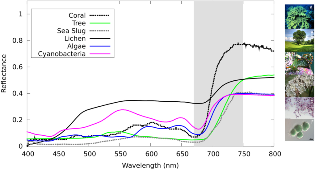
But are atmospheric biosignatures the only way to tell if life exists on other planets? Short answer: absolutely not. Let’s take Earth as an example. If we imagine Earth as a directly imaged exoplanet and take spectra of the light it reflects, you’ll find that around near-infrared wavelengths (~700 nanometers or just past the red part of the visible light spectrum), the light reflected off of Earth increases sharply. This sharp increase is called the vegetation red edge and is caused by plant and ocean life on Earth’s surface as shown in Figure 2. This is made possible because chlorophyll (the thing that makes plants green) absorbs nearly all visible light but reflects near-infrared light. The vegetation red edge is an example of a surface biosignature. In today’s article, the authors determine if the vegetation red edge will be visible in spectra of Earth-like exoplanets!

Spectra of different sources of the vegetation red edge

Figure 2: Spectra of different sources of the vegetation red edge on Earth. The vegetation red edge is highlighted in gray where the spectra rapidly increase and then level off beyond the visible light part of the spectrum. Each color represents a different source with pictures of each source on the right-hand side of the plot. [O’Malley-James and Kaltenegger 2019]

Snapshots

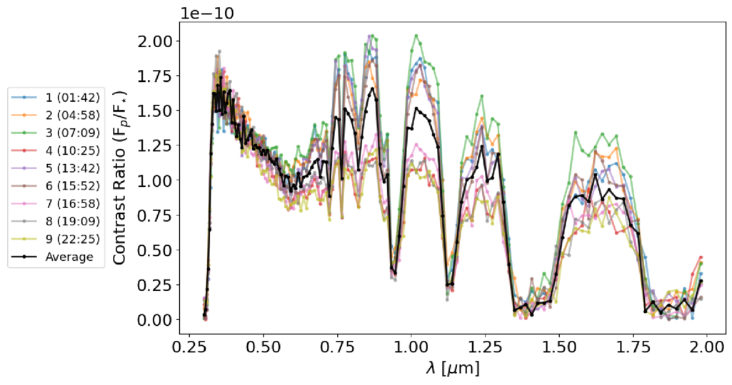
Planets rotate; that’s how we have morning, noon, and night in 24 hours guaranteed. This means that different parts of the surface will be visible at different times when we take spectra. Sometimes, we may see more ocean than land, other times not. To determine if the vegetation red edge would be visible at all points in Earth’s day, the authors simulated nine different spectra of modern-day Earth representing nine snapshots of Earth’s rotation. Additionally, they also simulated a time-averaged spectrum that shows an entire Earth day in one snapshot without the time variability. These spectra are shown in Figure 3.

Spectra of a directly imaged modern-day Earth at nine different times in its rotation

Figure 3: Spectra of a directly imaged modern-day Earth at nine different times in its rotation. The y-axis is the ratio of the planet’s signal to the star’s signal and the x-axis is wavelength in microns. Each color represents a time in UTC and the black curve represents the time-averaged spectrum. [Burr et al. 2026]

The authors then run retrieval models on all nine spectra to see if the vegetation red edge would be detectable in each spectrum, including the time-averaged one. Retrieval models take into account characteristics of the planet that would affect how light moves through its atmosphere, such as the atmospheric chemicals present and the surface gravity. They then use this information to generate possible spectral models that could fit the data. The best-fit model allows astronomers to infer what the atmosphere is made of and properties of the planet such as surface gravity. Because we are looking at Earth in visible light, much of the light from the planet is reflected. Typically, models of Earth-like planets in visible wavelengths only include atmospheric albedo: the measure of how reflective a planet’s atmosphere is. However, surface biosignatures can also be reflective as shown by the vegetation red edge. The authors use this to their advantage and introduce a surface albedo into their model that changes with the amount of desert, vegetation, and ocean visible on Earth’s surface at that time. They then further divide the nine spectra into three different types based upon the visible surface: majority land; 50% land, 50% ocean; and majority ocean. Check out the article online to see a cool animation of the Earth rotating and how the spectrum looks different at each time!

Arr! There Be… Vegetables?

After running the models, the authors were able to detect a sharp increase in the surface albedo value in every spectrum, including the time-averaged one. This result is shown in Figure 4. The authors take this result one step further in order to validate that the vegetation red edge is actually a result of surface variation of vegetation. They re-run models on each of their spectra but instead include a constant surface albedo instead of a time-varying one. This resulted in incorrectly measured radii, chemicals, and surface gravity in nearly all of the models. Without the vegetation red edge and surface features, the models could not accurately determine if life was present on Earth.

Retrieved surface albedos for the nine time-varying spectra

Figure 4: Retrieved surface albedos for the nine time-varying spectra. The surface albedo is broken down into three different values (a₁, a₂, a₃). Each of these values represents a change in the surface albedo at different wavelengths (i.e., how reflective the surface is at three different wavelengths). The nine spectra were broken down by the amount of surface that was visible at that time and color-coded for each category. The time-averaged spectrum is shown in gray. Each category of spectra was able to retrieve an increase in reflected light from the surface at vegetation red edge wavelengths. The spectra that had the majority land visible have the biggest increase in the surface albedo. This makes sense since the amount of visible vegetation is the largest with majority-land planets. [Burr et al. 2026]

For the first time (to the author’s knowledge), the vegetation red edge has been shown to be a promising and observable biosignature in Earth-like atmospheres. This study has also laid the groundwork for future work on other surface biosignatures and their potential impact on spectra of habitable planets. Confirming signs of life in multiple different ways, both on the surface and in the atmosphere, will finally allow astronomers to say we are not alone in the universe. In fact, life likes to live on the (red) edge!

Original astrobite edited by Madison VanWyngarden.

About the author, Kaz Gary:

I am a fourth-year PhD candidate at The Ohio State University with a passion for planets. My current work focuses on modeling exoplanet observations for the Habitable Worlds Observatory and understanding planetary atmospheres. Outside of research, I help develop planetarium shows and love all forms of science communication. In my free time, I enjoy playing tabletop RPGs, painting, watching terrible reality TV, and hanging out with my pet hedgehog.

The post Life on the (Red) Edge appeared first on AAS Nova.
Playing Pool with Planets

22 May 2026 at 17:00

artist's impression of hot Jupiter exoplanets

Each Jupiter-size planet in the galaxy falls into one of three distinct categories: hot, warm, or cold. A new study suggests that despite the apparent differences between these populations, they may have all formed from the same underlying dynamical process: a game of pool played at planetary scales.

A Diversity of Jupiters

Though our solar system has only one Jupiter-size planet, elsewhere in the galaxy we have found three different species of these massive gas giants. Cold Jupiters closely resemble their namesake and orbit far from their host stars; hot Jupiters are the opposite and are found whipping around their stars on extremely close-in orbits. In between these are the warm Jupiters, which tend to orbit in the intermediate space between 0.1 and 1.0 au.

A rendering of a star with lots of spots and flares with a planet in the foreground.

An artist’s depiction of a hot Jupiter. These planets orbit extremely close to their host stars, but likely got to their locations by scattering inward from more distant orbits. [NASA/JPL-Caltech]

Though these three populations are defined by their orbital distances, they differ from each other in other ways as well. For example, hot Jupiters almost never have nearby companions; if there are any other planets circling the same star, they’re usually far-out cold Jupiters. They can also orbit in pretty much any direction, including opposite the direction of their star’s spin, and are usually on perfectly circular orbits. In contrast, warm Jupiters often have friends nearby, are much more aligned with their stars’ spins, and can have modest eccentricities.

Given these differences, it’s often thought that each of these populations arrived at its current location through different dynamical processes and that the history of the warm Jupiters is likely quite different from the history of the hot Jupiters. However, a new study led by Julia Esposito (Georgia Institute of Technology) has proposed an alternative view. Maybe these populations, though they appear different now, were all created by the same process: planet–planet scattering.

Virtual Planetary Billiards

A cartoon of Jupiters at different distances from the sun with labelled arrows flowing inwards and outwards from each.

A schematic showing where different planets ended up as a function of where they scattered from during their evolution. Click to enlarge. [Esposito et al. 2026]

Esposito and collaborators set up 1,500 virtual planetary systems with three massive planets each, then simulated how the orbits evolved before probing the final configurations. In crucial contrast to previous simulation studies, the team initialized their Jupiters across a range of different distances and included the effects of tides sapping energy from orbits of planets that got too close to their host stars.

At the end of the simulation, the team surveyed the digital carnage. Almost every virtual system ended with only two planets after either ejecting one away from the star or having two planets collide. But, remarkably, the remaining two-planet systems looked tantalizingly similar to what we actually observe, with a mix of hot, warm, and cold Jupiters. Even more exciting, the end populations were highly correlated to where the violent scattering event took place.

For example, the warm Jupiters were almost all produced by “warm scattering” simulations, where the scattering took place between 0.1 and 1.0 au. The planets that survived the simulations and ended up as warm Jupiters matched all of the properties of the real warm Jupiter population: they had nearby companions, were moderately eccentric, and were mostly aligned with their stars. The hot Jupiters, meanwhile, were almost all produced by “cold scattering” events where the flybys happened far from the star and resulted in one planet hurtling inwards. These also matched all of the observed properties of real hot Jupiters.

The researchers concluded that planet–planet scattering can produce both the warm and hot Jupiter populations so long as you let the planets scatter from a variety of different distances. This exciting theoretical insight, if correct, would mean that astronomers could stop searching for different pathways to create each population. Happily, this model also provides testable predictions, and the authors lay out how the theory could be supported or disproven with additional data. Through virtual experiments like these, astronomers continue to build up an understanding of how the wide range of planetary architectures observed across the galaxy came to be.

Citation

“Unified Formation Channel of Hot and Warm Jupiters via Planet–Planet Scattering,” Julia Esposito et al 2026 ApJL 1003 L3. doi:10.3847/2041-8213/ae61b0

The post Playing Pool with Planets appeared first on AAS Nova.
Asteroid 2024 YR4 Won’t Hit the Moon, New JWST Observations Show

20 May 2026 at 17:00

asteroid 2024 yr4

Discovered in December 2024, the roughly 60-meter-wide asteroid 2024 YR4 was initially thought to have a slim chance of striking Earth in 2032. Further observations ruled out an Earth impact but left open the possibility of a Moon impact. New JWST observations show that 2024 YR4 will speed past both Earth and the Moon without a collision.

Another Update on 2024 YR4

In April 2025, we featured a Research Note that described March 2025 JWST observations of 2024 YR4 and characterized the asteroid’s size and albedo. At the close of that article, the authors suggested that further JWST observations in early 2026 could help to refine our understanding of the asteroid’s trajectory and determine whether it would strike the Moon.

On 18 and 26 February 2026, JWST carried out those critical observations. In this dataset, the asteroid is bright enough to be detected confidently, and the background is peppered with a sufficient number of reference stars — two factors necessary to determine the precise track of the asteroid as it zipped through space.

Trajectory Refinement

Difference between estimated and observed position for 2024 YR4

Difference between the position of 2024 YR4 determined in this work using three different reduction methods (red, blue, and green circles) and the position drawn from the existing orbit from the JPL Horizons database. The different analysis methods yielded consistent results. [Adapted from De Wit et al. 2026]

Julien de Wit (Massachusetts Institute of Technology) and collaborators analyzed the new JWST data and determined the asteroid’s position. The team used multiple methods to reduce the data and showed that their results were consistent regardless of the reduction method, ultimately yielding a measurement with an uncertainty of just 50 milliarcseconds. This is a huge improvement over the previous trajectory estimate, which had an uncertainty of 700 milliarcseconds.

Combining the latest JWST observations with existing data stretching back to the asteroid’s discovery, de Wit and coauthors determined a new, highly precise orbit for the object — one that definitively shows that the asteroid will safely pass by the Moon at a distance of 22,900 ± 800 km in 2032. In addition to ruling out the upcoming lunar impact, the team also ruled out any collisions with Earth in the next 100 years. Phew!

2024 YR4 observed and estimated position

Position of 2024 YR4 as seen by JWST in February 2026 (white dashed circle) compared to the asteroid’s location estimated from existing data (red circle). [De Wit et al. 2026]

High-Impact Science

This work highlights JWST’s potential as a tool for planetary defense. The February 2026 observations detailed here represent the faintest-ever detection of a near-Earth object, and JWST can detect objects far fainter than ground-based telescopes can. This ability allows JWST to observe potentially hazardous asteroids over a larger swath of their orbits, which translates to earlier trajectory estimation — JWST pinned down 2024 YR4’s orbit two years before the asteroid would have become bright enough for ground-based telescopes to do so.

JWST’s role may be even more important for smaller objects that rapidly become undetectable after discovery. De Wit’s team demonstrated this for a 10-meter-diameter 2024 YR4 clone on the same trajectory; for an object of this size, JWST would be able to rule out an Earth impact before the asteroid became undetectable, but ground-based telescopes could not. With surveys from facilities like Vera C. Rubin Observatory and Near-Earth Object Surveyor set to discover hundreds of thousands of new near-Earth objects, JWST’s role as a hazard assessor will likely be in high demand.

Citation

“JWST Observations of Asteroid 2024 YR4 Rule Out a 2032 Lunar Impact and Demonstrate a New Regime for Planetary Defense Follow-Up,” Julien de Wit et al 2026 ApJL 1003 L21. doi:10.3847/2041-8213/ae6a95

The post Asteroid 2024 YR4 Won’t Hit the Moon, New JWST Observations Show appeared first on AAS Nova.
I Spy with My Large Binocular Eyes: A Dusty Torus Around a Supermassive Black Hole?

19 May 2026 at 17:00

NGC 4151

Editor’s Note: Astrobites is a graduate-student-run organization that digests astrophysical literature for undergraduate students. As part of the partnership between the AAS and astrobites, we occasionally repost astrobites content here at AAS Nova. We hope you enjoy this post from astrobites; the original can be viewed at astrobites.org.

Title: Shocks, Winds, and a Torus: The Large Binocular Telescope Interferometer (LBTI) Resolves the Active Nucleus of NGC 4151
Authors: Jacob W. Isbell et al.
First Author’s Institution: University of Arizona
Status: Published in ApJ

At the centre of nearly every galaxy lies a supermassive black hole that dominates this innermost region. Not only is there this millions-of-solar-masses dark beast, but usually too a whole bunch of stuff — stars, gas, dust, and more — which is often quite bright! When there is plenty of this material quite close to the black hole, we believe physics takes control to flatten it into a family of disk and toroidal structures in what we call the unified model of active galactic nuclei (AGNs; see Figure 1).

schematic of the unified model of active galactic nuclei

Figure 1: The unified model of AGNs asserts that there is an inner accretion disk, surrounded by a dusty torus that cohabitates with clouds moving at different velocities (the so-called broad and narrow line regions), and sometimes even relativistic jets extending from the accretion disk to galactic scales; you can read more about AGN structure in this Astrobites guide. [Emma Alexander; CC BY 4.0]

When astronomers look at different active galaxies (read: galaxies with active supermassive black holes at their core), we see a range of phenomenologies related to their brightness, spectra, morphologies, and more. The unified model of AGNs seeks to explain these different AGN appearances simultaneously by positing that they all have the same physical structure, and we are just viewing them from different angles, hence seeing different features.

The cores of AGNs are often imaged at the smallest scales (e.g., their accretion disks, viewed with interferometers like the Very Large Telescope Interferometer) and the largest scales (e.g., their relativistic jets, viewed with radio interferometers), but comparatively less effort has gone to directly observing the predicted dusty tori in the mid-infrared. That is exactly what today’s authors set out to do using the Large Binocular Telescope Interferometer (LBTI) — a pair of 8.4-metre-aperture mirrors separated by just over 14 metres and combined to simulate a telescope effectively 29 metres wide. This lets astronomers take direct images at a much higher resolution than a smaller-aperture telescope, and hence directly peer into the region around AGNs where this dusty torus should lie.

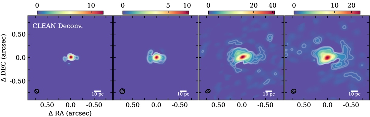
Today’s authors turn the LBTI towards NGC 4151, a medium-luminosity AGN. With the large effective aperture of the LBTI, they were able to resolve scales in the AGN region as small as 4.4–9.1 pc, about 14–30 light-years depending on the wavelength (see Figure 2), in the mid-infrared. These observations revealed warm dust emission in a complex structure around the central supermassive black hole. The authors note a central bar at all wavelengths, with a significant extension of cool dust arcing to the west (right in the image) and warmer dust localised to the centre (as evident by 3.7- and 4.8-micron emission only nearest to the supermassive black hole and its accretion disk).

deconvolved images of the AGN core of NGC 4151

Figure 2: The deconvolved images of the AGN core of NGC 4151 show a very bright central source (the innermost region around the supermassive black hole), as well as some complex surrounding structure particularly at long wavelengths. The interpreted morphology is described in Figure 3. These images are deconvolved, meaning that known optical effects are corrected for on the raw data to produce a sharper image. [Adapted from Isbell et al. 2026]

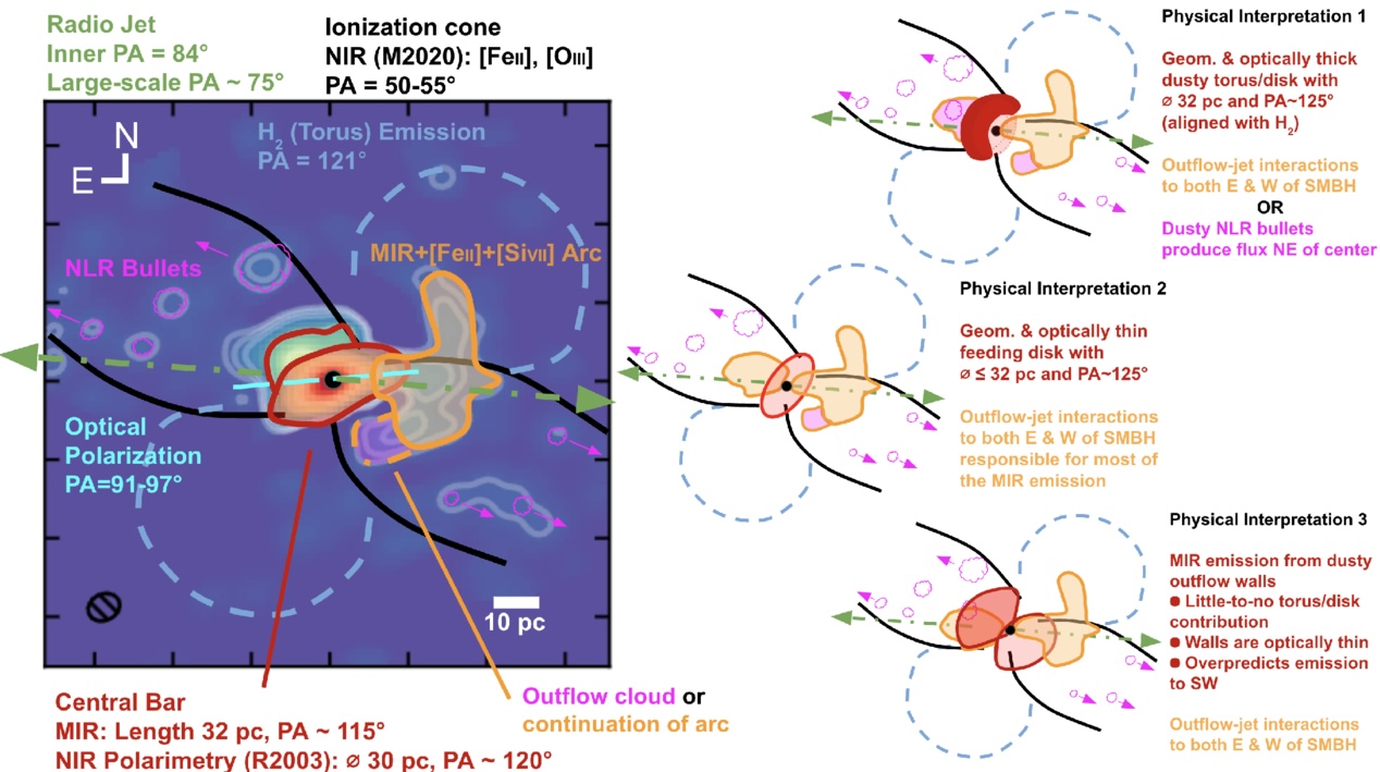
To explain the observed morphology in Figure 1, the authors compare three different interpretations based on this new high-resolution imagery together with the results of previous studies looking at other scales and the spectrum of the AGN core. Each interpretation is illustrated and briefed in Figure 3.
illustration of the different regions surrounding NGC 4151's black hole and potential interpretations for the observed morphology

Figure 3: Three interpretations of the observed morphology are presented by the authors. The left panel illustrates the different regions surrounding the supermassive black hole (together with the results of other studies cited in the article). The right panel shows the suggested interpretations explaining the morphology. [Isbell et al. 2026]

The first interpretation is in keeping with the unified model of AGNs: a geometrically and optically thick torus of dust surrounds the inner region. In this interpretation, the surface of the dusty torus re-radiates light from the accretion disk to produce most of the mid-infrared emission. Additional mid-infrared emission could come from localised concentrations of gas or interactions between the outflow and the jet. The authors immediately disfavour this explanation, as other studies have shown bright ionised emission at the location of the would-be torus, which is not expected if an optically thick torus were to be present. Hence, these new observations somewhat challenge the one “flavour” of the unified model of AGNs.

The second interpretation aligns with a different version of the unified model: one in which a geometrically thin disk replaces a thick torus around the AGN core. Provided the disk is optically thin too, the authors favour this approach as it is consistent with the geometry of ionised emission that worked against the first interpretation. While other studies suggest that this thin disk should be optically thick, this morphology is at least better aligned with what we see in other AGNs.

The third interpretation suggests that the emission comes from only the radiation pressure–driven wind emanating from the AGN core. The authors disfavour this explanation, citing previous radiative transfer simulations that show that the flux should fall off with distance from the core too quickly to be consistent with the observations.

No matter the interpretation, these LBTI observations are an important glimpse into the future of mid-infrared AGN studies that will be done with 30-metre-class telescopes (such as the European Southern Observatory’s Extremely Large Telescope). This article, together with the group’s similar study on NGC 1068, is challenging and refining an accepted view of AGN morphology — the consequences of which apply to galaxies near and far — and poses new questions perfect for sophisticated hydrodynamic and radiative simulations.

Original astrobite edited by Margaret Verrico.

About the author, Ryan White:

I am a first-year PhD student at Macquarie University in Australia, working mainly on binary/multiple systems with massive stars (Wolf–Rayets in particular!). Outside of study, I’m probably drinking coffee, baking, reading, or going for a run. You can also find me procrastinating on Bluesky @astroryan.bsky.social.

The post I Spy with My Large Binocular Eyes: A Dusty Torus Around a Supermassive Black Hole? appeared first on AAS Nova.
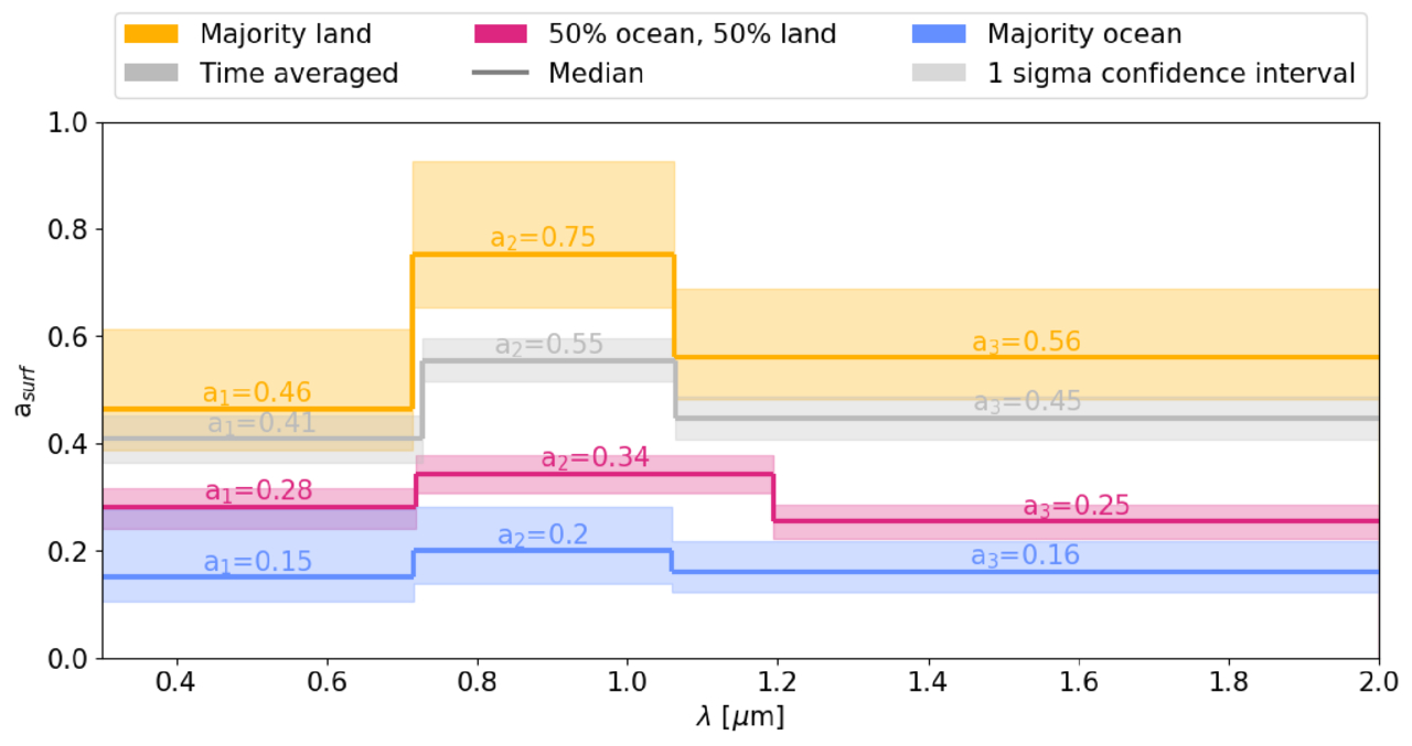
Featured Image: Chasing Weywot’s Shadow

18 May 2026 at 17:00

graphics showing the predicted and actual paths of Weywot's stellar occultations

The outer solar system is inhabited by swarms of small objects that are challenging to observe and characterize. When one of these objects travels in front of a star, from our perspective, the passage provides a brief chance to study these distant, icy denizens of our solar system. In a recent article, Estela Fernández-Valenzuela (University of Central Florida) and coauthors described how they predicted and observed stellar crossings by Weywot, the largest moon of the dwarf planet Quaoar, which lies roughly 44 au from the Sun. In the image above, the black dashed lines indicate the areas where Weywot was predicted to briefly blot out the light from a star, and the blue lines show the updated regions based on Hubble Space Telescope observations. In each panel, the green squares and red circles show where the occultation was and was not detected, respectively. There were five successful detections of Weywot’s passage across a star, allowing the team to constrain Weywot’s diameter to 116–172 km. The team also found that Weywot is much darker than the body it orbits, which has important implications for how the system formed. To learn more about the planning process for and results of these observations, be sure to check out the full research article linked below.

Citation

“Weywot, an Unusually Low-Albedo Satellite in the Trans-Neptunian Region,” Estela Fernández-Valenzuela et al 2026 ApJL 1002 L37. doi:10.3847/2041-8213/ae6076

The post Featured Image: Chasing Weywot’s Shadow appeared first on AAS Nova.
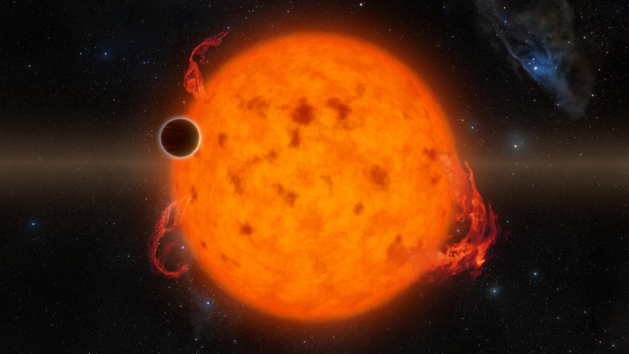
Hints for Massive Galaxy Evolution from Dusty Star-Forming Galaxies

15 May 2026 at 17:00

NGC 972

How do massive galaxies form and evolve? A recent study traces the stellar and dust distributions across evolutionary phases of massive galaxies to better understand how massive dusty star-forming galaxies fit into the picture.

Dusty Massive Galaxies

Massive galaxies, like the Milky Way or even larger, undergo phases of active star formation and quiescent phases of inactivity, but exactly how these galaxies evolve through these stages is not yet fully understood. Dusty star-forming galaxies, which are undergoing a period of intense star formation and shrouded in dust, might be the missing evolutionary step between star-forming and quiescent phases of massive galaxy evolution. 

Currently, the leading explanation for massive galaxy formation and evolution is inside-out growth — star formation and quenching start in the inner regions of a galaxy and progress outward. However, it’s not clear whether dusty star-forming galaxies also follow the favored inside-out pathway, or if they instead proceed outside-in, first growing their disks and then assembling a central bulge.

JWST NIRCam images

Example of JWST NIRCam images with ALMA contour lines overlaid for select dusty star-forming galaxies in the sample. [Modified from Bodansky et al 2026]

The spatial distribution (or morphology) of the stars and dust within dusty massive galaxies can help us trace their evolution. Thanks to high-resolution observations from JWST and the Atacama Large Millimeter/submillimeter Array (ALMA), researchers can now directly compare the morphologies of distant star-forming, quiescent, and dusty galaxies during the height of our universe’s star formation. Filling this gap will reveal how dusty star-forming galaxies may connect star-forming and quiescent galaxies in massive galaxy evolution.

Multiwavelength Morphological Comparisons

To directly compare the star and dust morphologies across massive galaxies, Sarah Bodansky (University of Massachusetts, Amherst) and collaborators selected a sample of 33 dusty star-forming galaxies from the GOODS-ALMA 2.0 survey that searched the sky for 1.1-mm dust emission as well as star-forming and quiescent comparison samples drawn from JWST observations. Combining the ALMA survey data with JWST imaging, the authors studied the rest-frame optical (stars) and rest-frame near-infrared (dust) morphologies of dusty, star-forming, and quiescent galaxies at redshifts around cosmic noon (a few billion years after the Big Bang).

When comparing optical morphologies, the authors found that dusty star-forming galaxies and typical star-forming galaxies had similar distributions, but their near-infrared morphologies showed clear differences. Dusty galaxies tended to show more compact near-infrared emission, with dust tracing their stellar populations and more concentrated in the galaxies’ central regions. Though clearly different from star-forming galaxies, the authors noted striking similarities between the near-infrared morphologies of the dusty star-forming and quiescent galaxies, especially within their centers.

Surface brightness profiles

Average surface brightness profiles for the rest-optical (left) and rest-near-infrared (right) for the dusty (black), star-forming (blue), and quiescent (red) galaxies. In the near-infrared, the dusty star-forming galaxy profile appears very similar to the quiescent galaxy profile. [Bodansky et al 2026]

All of these properties suggest that dusty star-forming galaxies have built up stellar mass and dust in their cores, potentially forming a central bulge first and supporting an inside-out model of massive galaxy growth. This points to dusty star-forming galaxies as possible direct progenitors of early massive quiescent galaxies, hanging onto their last bit of star formation before becoming quiet as well. While this study morphologically distinguishes dusty galaxies from their star-forming and quiescent counterparts, future spectroscopic studies comparing the kinematics of these populations and investigations of molecular gas distributions are necessary to better pin down the evolutionary connection between star-forming, dusty, and quiescent massive galaxies.

Citation

“JWST+ALMA Reveal the Buildup of Stellar Mass in the Cores of Dusty Star-forming Galaxies at Cosmic Noon,” Sarah Bodansky et al 2026 ApJ 1001 235. doi:10.3847/1538-4357/ae4f64

The post Hints for Massive Galaxy Evolution from Dusty Star-Forming Galaxies appeared first on AAS Nova.
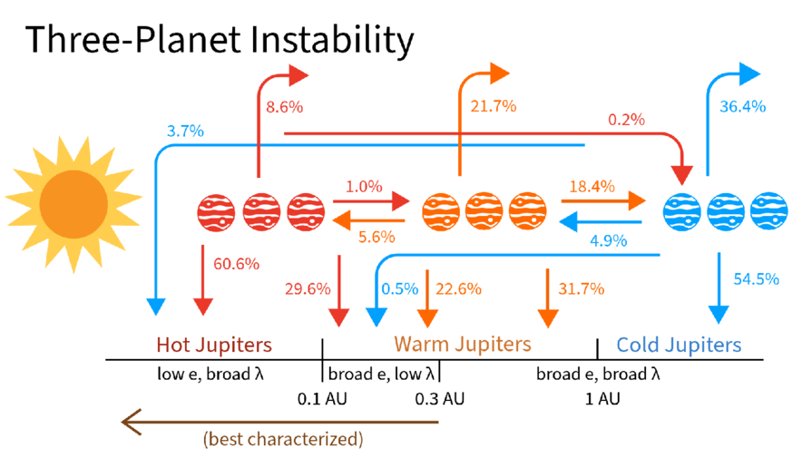
Interstellar Comet 3I/ATLAS Through the Eyes of Rubin Observatory

13 May 2026 at 17:00

Rubin Observatory with star trails

The NSF–DOE Vera C. Rubin Observatory has yet to begin its 10-year Legacy Survey of Space and Time, but it’s already keeping an eye on the sky. Astronomers recently described Rubin’s serendipitous spotting of 3I/ATLAS days before the interstellar object’s discovery.

3I/ATLAS

Interstellar comet 3I/ATLAS as seen by the Hubble Space Telescope on 30 November 2025. [NASA, ESA, STScI, D. Jewitt (UCLA), M.-T. Hui (Shanghai Astronomical Observatory). Image Processing: J. DePasquale (STScI)]

Welcome, 3I/ATLAS

Our solar system has been playing host to a rare interstellar tourist: 3I/ATLAS. Just the third known interstellar object to have passed through our star system, 3I/ATLAS was discovered on 1 July 2025 by the robotic telescope network of the Asteroid Terrestrial-impact Last Alert System (ATLAS). After making its closest approach to the Sun in October 2025, 3I/ATLAS is now journeying out of the solar system and is currently located beyond the orbit of Jupiter.

While astronomers would likely grumble about hosting a human guest for nearly a year, they’ve been thrilled with 3I/ATLAS’s lengthy visit and have turned countless telescopes toward the rare interstellar object. They’ve also turned to the archives, searching for pre-discovery sightings of the object — and finding them in the commissioning data from one of the most highly anticipated observatories on the planet: Rubin Observatory.

A Serendipitous Sight

3I/ATLAS from Rubin Observatory

3I/ATLAS as seen by Rubin Observatory on 3 July 2025. [Chandler et al. 2026]

In the months since the release of Rubin’s exceptional first images, its 8.4-meter telescope and array of instruments have undergone rigorous testing to ensure they can meet the high standards required for the upcoming survey.

For most of 2025, Rubin was in its commissioning phase, carrying out science validation observations — a critical period during which instruments, procedures, and pipelines are fine tuned, and the quality and quantity of data collection can vary. On 20 June 2025, the very first night of its science validation survey, Rubin happened to turn toward the small patch of sky containing the as-yet undiscovered 3I/ATLAS.

More to Come

In a recent article, Colin Orion Chandler (LSST Interdisciplinary Network for Collaboration and Computing Frameworks; University of Washington) and collaborators described how they tracked down 3I/ATLAS in Rubin’s commissioning data after the object’s discovery was announced. In total, the observatory serendipitously spotted 3I/ATLAS nine times between 21 June and 2 July, then several more times — some on purpose, some by chance — between 3 and 20 July.

Serendipitous observations of 3I/ATLAS by Rubin

Serendipitous observations of 3I/ATLAS by Rubin. [Chandler et al. 2026]

Analyzing Rubin’s observations of 3I/ATLAS required the development of custom techniques, since the observatory’s pipeline for handling observations of rapidly moving solar system objects was not in operation at that time. Despite these challenges, Chandler’s team successfully made astrometric measurements, collected photometry, determined 3I/ATLAS’s orbit, and studied the comet’s structure and nucleus. Among other findings, these data clearly show the presence of the object’s fuzzy coma, providing the earliest high-resolution evidence of cometary activity.

In their analysis of Rubin’s observations of 3I/ATLAS, Chandler and collaborators found that had the science validation survey started sooner, and had the analysis pipelines been operational, Rubin might have been the first to welcome humanity’s third interstellar visitor. Findings like these heighten the anticipation for the start of the Legacy Survey of Space and Time, during which Rubin will surely build upon its already impressive record of interstellar object observations.

Citation

“NSF-DOE Vera C. Rubin Observatory Observations of Interstellar Comet 3I/ATLAS (C/2025 N1),” Colin Orion Chandler et al 2026 ApJL 1001 L35. doi:10.3847/2041-8213/ae4b3a

The post Interstellar Comet 3I/ATLAS Through the Eyes of Rubin Observatory appeared first on AAS Nova.
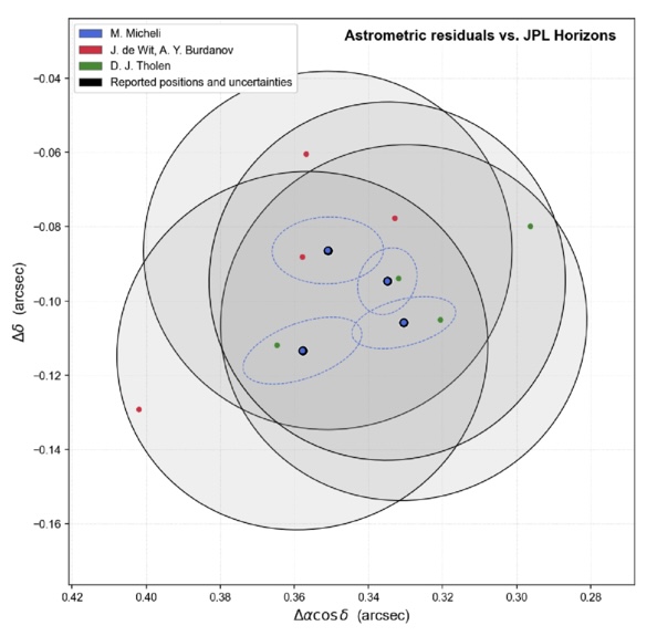
Hunting for Exomoons Around a Lonely Planet

12 May 2026 at 17:00

illustration of an exoplanet and exomoon around a star

Editor’s Note: Astrobites is a graduate-student-run organization that digests astrophysical literature for undergraduate students. As part of the partnership between the AAS and astrobites, we occasionally repost astrobites content here at AAS Nova. We hope you enjoy this post from astrobites; the original can be viewed at astrobites.org.

Title: A Deep Search for Exomoons Around WISE 0855 with JWST
Authors: Mikayla J. Wilson et al.
First Author’s Institution: University of California, Santa Cruz
Status: Published in AJ

The “Moon”-umental Question

The solar system hosts hundreds of moons, ranging from volcanic worlds like Io around Jupiter, to icy objects like Enceladus around Saturn, to captured objects like Neptune’s retrograde moon Triton. Moons are essential to our model of how the solar system formed and also offer some of the best chances we have for finding life beyond Earth.

Astronomers also expect exomoons, or moons orbiting planets outside the solar system, to be abundant around other giant exoplanets. But how common are exomoons? How do they compare to the moons in our solar system?

In order to begin answering those questions, we must first detect an exomoon, which has proved difficult despite decades of searching by astronomers. Fortunately, JWST presents a new opportunity to uncover the exomoon population by looking at lonely free-floating planets as they drift through space.

Why Free-Floating Planets?

One proposed method for searching for exomoons is by looking for their transits in front of their host planets, characterized by the dips in brightness of the planet as the moon passes in front, blocking the planet’s light. Looking for exomoon transits around planets orbiting stars is quite difficult, as the bright starlight can easily drown out the small signals of exomoon transits. Free-floating planets solve this issue by removing the star entirely, increasing our sensitivity to such detections. (See this bite for a good review.)

The authors of today’s article directed the exomoon hunt towards the free-floating WISE J085510.83-071442.5 (or WISE 0855). It has the prestige of being the coldest known brown dwarf (250–285K) while also sitting at a relatively low mass (3–10 Jupiter masses). Notably, it is also one of our closest neighbors at a distance of only 7.4 light-years, making it ideal for high-precision observations despite its faintness. Even though brown dwarfs are technically distinct from planets, the authors opt to refer to companions around WISE 0855 as moons given WISE 0855’s “planetary-mass” status. (It’s complicated…)

Repurposing JWST Data… for Moons!

The JWST observations used in this study contain 11 hours of near-infrared (2.87–5.27 microns) time-series spectra originally intended to study water clouds and weather on WISE 0855. Time-series brightness monitoring can also be used for transit searches, which the authors take advantage of.

One complication is that WISE 0855 is variable, meaning its intrinsic brightness changes over time. Variability is likely driven by clouds and other dynamic processes within its atmosphere. So how do the authors distinguish between a passing moon and a turbulent atmosphere? The key idea is that variability is wavelength dependent, meaning that the brightness of WISE 0855 will fluctuate differently depending on the observed wavelength. In contrast, transits are “gray,” meaning that the same amount of light is blocked at all wavelengths, producing a consistent feature across the entire spectrum.

Finding Moons with Statistics!

The authors apply this idea and pick out two wavelength regions of WISE 0855’s spectrum that contain two distinct variability patterns, which should both contain an identical moon transit signal (if present). They then generate a light curve (how brightness changes over time) for these two regions (see Fig. 1).

WISE 0855 light curves

Figure 1: (A) Light curves from two selected wavelength regions of WISE 0855’s spectrum with injected transit signals. Also plotted is the best-fit Gaussian processes + transit model for the two light curves. (B) Light curve data after subtracting the Gaussian processes portion of the best-fit model, revealing the example injected transit signals. [Wilson et al. 2025]

To appropriately model the variability, the authors employ Gaussian processes, a flexible tool that can model complex, quasi-periodic signals like atmospheric variability. They compare fits from two types of models:
  • Gaussian processes–only model: Assumes that all observed variability is intrinsic to the planet itself
  • Gaussian processes + transit model: Includes a simple trapezoidal exomoon transit signal that is simultaneously fit in both light curves

Using Bayesian evidence (a measure of how well each model explains the data), they determined which model was favored. So, what do they find?

The Bad News and the Good News

Based on Bayesian evidence, the authors conclude that there are no statistically significant detections of exomoons in the data. The results suggest very weak evidence for a ~0.53-Earth-radius moon at a wide separation from WISE 0855 — an unlikely scenario given that transit probability decreases at greater separations (and therefore longer orbital periods).

Yet, the study goes further: What kinds of moons is JWST able to detect, if any? To answer this, the authors performed injection and recovery tests, where they injected artificial transit signals of varying depths (exomoon sizes) into the data and tested how well their models were able to recover them (results shown in Fig. 2). They find that JWST is capable of detecting 96% of transits with depths ≥0.5%, equivalent to a Titan-like moon. Smaller Io-like moons were also detectable more than half of the time. This means that if a Titan analog had actually transited during these observations, we would almost certainly have seen it!

plot of successful detections of injected transit signals

Figure 2: Results showing the number of successful detections for the transit injection and recovery tests. Fifty transit injections are done for transit depths of 1%, 0.5%, 0.4%, 0.3%, 0.2%, and 0.1%. The transit depths represent different exomoon sizes, with the shaded regions representing Io-like and Titan-like moons. [Wilson et al. 2025]

JWST will continue to gather more time-series data of free-floating planets, brown dwarfs, and directly imaged exoplanets, each providing a new opportunity to help us better understand the moon population outside of our solar system. We’re still waiting for the first confirmed exomoon, but when that transit finally happens, we know that JWST will be ready.

Original astrobite edited by Kelsie Taylor.

About the author, Jared Bull:

I am a 2nd-year PhD student at Johns Hopkins University. I study brown dwarf variability and am interested in using time-series observations to uncover dynamic processes within their atmospheres. In my free time I like to read, cook, and do astrophotography.

The post Hunting for Exomoons Around a Lonely Planet appeared first on AAS Nova.
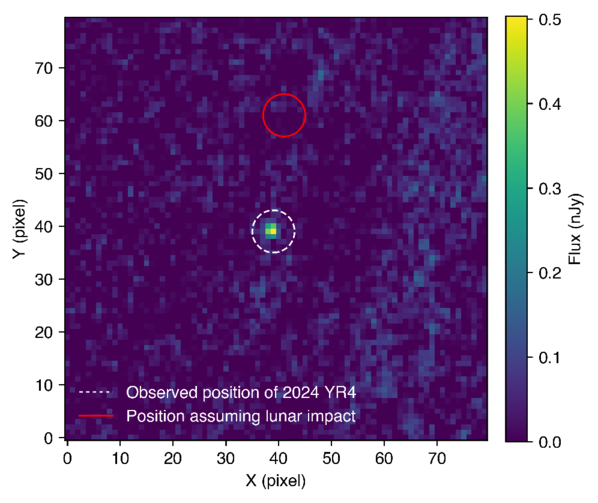
Into the Void: Investigating the Heart of a Giant Elliptical Galaxy

11 May 2026 at 17:00

giant elliptical galaxy

The core of the brightest galaxy in the cluster Abell 402 contains a curious void. New observations suggest that an ultra-massive black hole could have excavated this feature.

At the Center of the Center of a Cluster

JWST and Hubble observations of A402-BCG

JWST and Hubble observations of A402-BCG. In addition to the dark cavity previously seen by Hubble, the galaxy’s center hosts an infrared-bright source. Click to enlarge. [McDonald et al. 2026]

Abell 402 is a galaxy cluster located roughly 4 billion light-years away, and at its center is a giant elliptical galaxy called A402-BCG. Zooming in on the heart of this galaxy, astronomers using the Hubble Space Telescope discovered a dark region that they suspected was due to a cloud of dust blocking the starlight from the galaxy’s center.

In a recent research article, a team led by Michael McDonald (Massachusetts Institute of Technology) investigated this dark region to test the dust-cloud hypothesis and explore other explanations.

McDonald’s team compiled new JWST Near-Infrared Camera data, archival Hubble imaging, and spectroscopy from the Multi Unit Spectroscopic Explorer (MUSE) on the Very Large Telescope. The new JWST images show a prominent dark feature at the center of A402-BCG, plus a bright source directly beside it.

comparison of A402-BCG to Abell 1060

Comparison of the cavity in A402-BCG (bottom row) to the dust ring in Abell 1060’s central galaxy (top row). In the middle row, simulated observations show Abell 1060’s central galaxy at A402-BCG’s redshift. The appearance of the dust ring is wavelength dependent, but the appearance of A402-BCG’s cavity is not. [Adapted from McDonald et al. 2026]

Not Hidden, but Missing

If the dark feature at the center of A402-BCG is a dust cloud, the cloud would be less obscuring at the near-infrared wavelengths captured by JWST than at the optical wavelengths sampled by Hubble. However, the feature was equally dark in the JWST images, leading the team to rule out the dust-cloud hypothesis.

Instead, they favor a scenario in which the dark feature is due to an absence of stars rather than the presence of obscuring dust. The team estimated that 2 billion solar masses of stars are missing — equivalent to 1% of the stellar mass of the galaxy. What’s more, the cavity is situated in a larger region of constant surface brightness called a core, in which there are fewer stars than expected.

The Dynamical History of A402-BCG

McDonald and coauthors suggested that the missing stars in A402-BCG’s core and cavity were ejected by at least one supermassive black hole binary. They estimated that the core region, which is roughly 6,500 light-years across, was excavated by a 50 billion solar mass black hole. This epic black hole may be the result of a past merger and is likely located at the infrared-bright spot on the border of the cavity, as this source’s spectral energy distribution resembles that of an actively accreting black hole.

MUSE observations showing ionized gas within A402-BCG

MUSE observations of highly ionized gas in A402-BCG. The blueshifted source on the right coincides with the infrared-bright source, while the redshifted source on the left appears to be embedded within a larger ionized envelope. [Adapted from McDonald et al. 2026]

MUSE spectroscopy provided evidence for a second black hole. These data revealed two pockets of ionized gas — one coincident with the infrared-bright source, the other on the opposite side of the cavity — as well as two distinct sets of emission lines consistent with a black hole binary totaling 60 ± 20 billion solar masses. (The team noted that alternate explanations for the second source, like a compact starburst, were less likely but couldn’t be ruled out.)

The team favors a scenario in which these black holes are slowly spiraling toward one another, ejecting stars from the galaxy’s center as they move and carving out a deep deficit of stars. This stellar cavity sits within a larger region of stellar scarcity that was scooped out by a past supermassive black hole merger that created the ultra-massive black hole present in the galaxy today. Simulations suggest that only about 0.5% of massive galaxies are in this phase of evolution at a time, so we may have caught A402-BCG in a fascinating moment — one that provides new clues about how to search for ongoing black hole mergers in other galaxies.

Citation

“A Kiloparsec-Scale Stellar Cavity in the Center of A402-BCG May Be Caused by Dynamic Interactions with an Ultramassive Black Hole,” Michael McDonald et al 2026 ApJL 1002 L19. doi:10.3847/2041-8213/ae5bbe

The post Into the Void: Investigating the Heart of a Giant Elliptical Galaxy appeared first on AAS Nova.
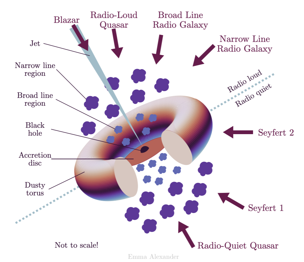
❌