❌

Normal view

Monthly Roundup: Science of the Sun

27 April 2026 at 17:00

three images of the Sun

The Sun’s activity history, the sources of tiny jets, and how magnetic fields might impact space weather forecasts: today’s Monthly Roundup introduces a trio of recent research articles from the Astrophysical Journal that tackle hot topics in solar physics.

From 1755 to 2020: Reconstructing Centuries of Solar Activity

Since the 1970s, regular monitoring of the Sun’s magnetic field has allowed researchers to decipher the Sun’s behavior as it cycles through periods of low and high activity. But what resources exist for studying the Sun’s past behavior? To investigate the long-term behavior of the Sun, researchers reach for historical records of sunspots, which stretch back to the 1700s.
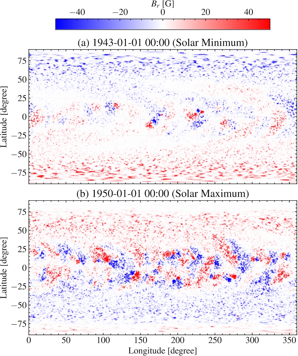
maps of simulated photospheric magnetic fields

Example maps of the simulated photospheric radial magnetic field during a period of low (top) and high (bottom) solar activity. Click to enlarge. [Jha et al. 2026]

Bibhuti Kumar Jha (Southwest Research Institute) and collaborators explored whether historical records and modern statistics could be used to reconstruct the behavior of the solar magnetic field centuries into the past. Jha’s team used recorded sunspot numbers from 1755 to 2020 as an input for their newly developed Synthetic Active Region Generator, which generates synthetic solar active regions based on known statistics of these regions. This catalog of active regions becomes the input for the Advective Flux Transport model, which simulates the active regions as they emerge and evolve, allowing for an estimation of the magnetic field across the Sun’s disk.

Jha and coauthors found that this method successfully reproduced the expected large-scale behavior of the Sun’s magnetic field across multiple solar cycles, such as the reversal of the polarity of the solar magnetic field near the peak of the activity cycle. While this work highlights the impressive results obtained from combining historical sunspot records with modern sunspot statistics, the team pointed out that this method cannot accurately reproduce all quantities because of the nonlinear nature of the underlying physics. Future work will refine the model further, and in the meantime, the team’s simulated historical magnetic field maps will be made publicly available.

Where Do the Tiniest Coronal Jets Come From?

The Sun’s atmosphere is filled with an ever-shifting maze of magnetic field lines, which reconfigure and release pent-up magnetic energy in a process calledΒ magnetic reconnection. Magnetic reconnection can launch particles and heat plasma, and it’s thought to be responsible for driving jets on a variety of scales in the Sun’s tenuous outer atmosphere, or corona. Annu Bura (Indian Institute of Astrophysics; Pondicherry University) and coauthors investigated the physical origins of the smallest of these reconnection driven jets, picoflare jets, using data from the Extreme Ultraviolet Imager on board Solar Orbiter. Solar Orbiter has ventured within 0.3 au of the Sun, and its Extreme Ultraviolet Imager has returned exceptionally precise high-energy images of our home star.
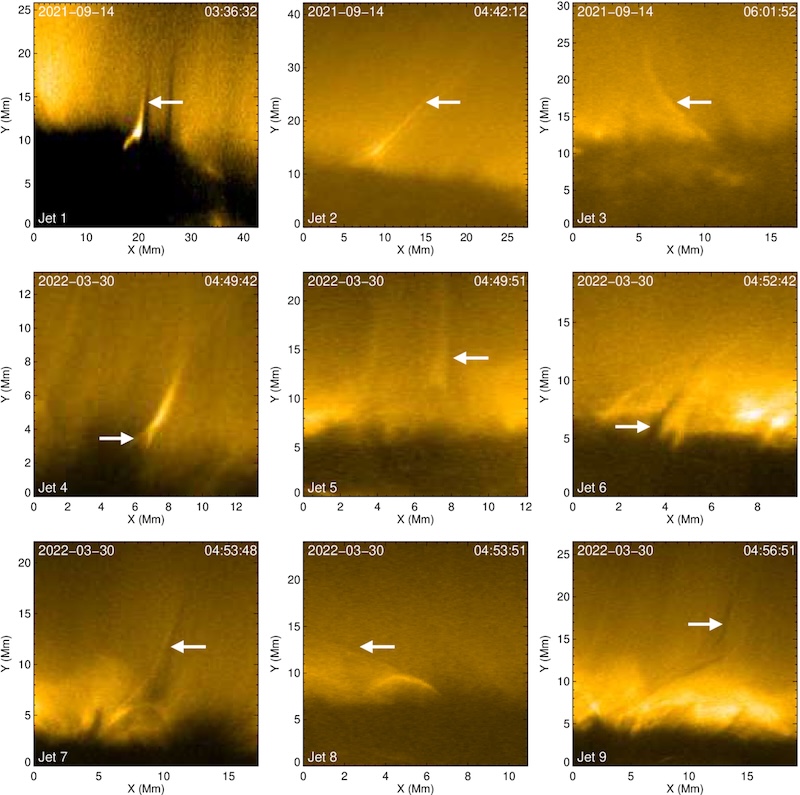
Examples of coronal jetlets

Examples of jets identified in this study. You can see an animation of this figure. [Bura et al. 2026]

Bura and collaborators identified picoflare jets by the presence of a hot, bright spire coupled with a cool, dark streak, forming a structure shaped like the letter β€œY” upside down. They found that the bright and dark features were on average 650 and 490 kilometers wide, respectively, with a typical jet length of 16,900 kilometers. They also found that the bright features moved more quickly than the dark features, and the jets tended to last about 6 minutes. Overall, these measurements place the jets in between the scales expected for picoflare jets and slightly larger features called jetlets, though the energies are consistent with expectations for picoflare jets.

Using radiation magnetohydrodynamics simulations, the team explored the origins of their sample of jets. The simulations suggested that the bright features arose from hot, tenuous coronal plasma, while the accompanying dark features were due to cooler, denser plasma venturing upward from deeper in the Sun’s atmosphere, in the chromosphere. Overall, the simulations and observations support a picture in which picoflare-scale jets are driven by magnetic reconnection after magnetic flux emerges through the Sun’s surface. This echoes the formation route of larger coronal jets, suggesting that this process may apply to a wide range of physical scales.

Investigating the Influence of the Solar Polar Magnetic Field

The vast majority of our observations of the Sun have come from within a few degrees of the ecliptic plane, either from telescopes situated on Earth’s surface or from spacecraft that stuck close to the plane of our solar system. With rare but notable exceptions β€” the Ulysses spacecraft, which measured the Sun’s magnetic field and plasma environment from a near-polar orbit, and Solar Orbiter, which took the first-ever image of the Sun’s poles in November 2025 β€” the Sun’s poles have remained hidden from our instruments.

Our limited knowledge of the Sun’s polar magnetic field has consequences for our ability to model space weather events like coronal mass ejections. A team led byΒ Xiao Zhang (Chinese Academy of Sciences; University of Chinese Academy of Sciences) has used numerical simulations to investigate how solar polar magnetic field conditions influence the propagation of a coronal mass ejection (CME) through the solar system.
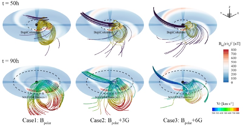
Simulation results showing the propagation and expansion of a coronal mass ejection

Simulation results showing how the propagation and expansion of a CME are affected by the polar magnetic field strength. Click to enlarge. [Zhang et al. 2026]

The team simulated a CME from 4 December 2021, which was observed by the BepiColombo spacecraft at Mercury and Tianwen-1 and MAVEN at Mars. The simulations showed that as the polar magnetic field strength increases, the CME’s movement through the solar system becomes slower. CMEs typically expand as they billow outward from the solar corona and sweep past the planets; increasing the polar magnetic field strength slowed the CME’s expansion as well. A stronger polar magnetic field also alters the background solar wind, making it slower and denser. Overall, these results demonstrate that the strength of the Sun’s poorly constrained polar magnetic field can have a significant impact on the movement and evolution of a CME. In future work, Zhang’s team plans to expand their investigation to a larger sample of CMEs.

Citation

β€œHistorical Reconstruction of Solar Surface Magnetism from Cycles 1–24 Using the Synthetic Active Region Generator and the Advective Flux Transport Model,” Bibhuti Kumar Jha et al 2026 ApJ 997 279. doi:10.3847/1538-4357/ae279a

β€œOn the Origin of Coronal Picoflare Jets,” Annu Bura et al 2026 ApJ 1000 94. doi:10.3847/1538-4357/ae48e6

β€œInfluence of Solar Polar Magnetic Fields on the Propagation of Coronal Mass Ejections,” Xiao Zhang et al 2026 ApJ 1000 200. doi:10.3847/1538-4357/ae4c54

The post Monthly Roundup: Science of the Sun appeared first on AAS Nova.
Astronomers See Braided Magnetic Fields Above a Sunspot

11 March 2026 at 16:00

sunspot

Revealed in high resolution, researchers have spotted complex twisting and braiding motions in fine threads of plasma suspended above a sunspot. The flow of material that followed this braiding provides evidence for magnetic reconnection.

Heating Up the Corona

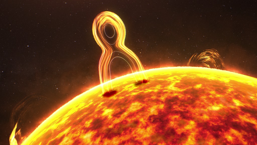
illustration of magnetic reconnection on the Sun

Magnetic reconnection is common throughout the universe, from Earth’s magnetic field to the jets of supermassive black holes. This illustration shows magnetic reconnection happening on the Sun. [NASA’s Conceptual Image Laboratory]

One of the leading challenges for the field of solar physics is explaining how the temperature of the Sun skyrockets from roughly 6000K at its surface, or photosphere, to more than 106K in its wispy corona. The top candidates for the resolution to this mystery are magnetohydrodynamic waves and magnetic reconnection, in which nearby field lines reorganize into a lower-energy configuration and release magnetic energy.

One way for magnetic reconnection to heat the corona is along magnetic fields that loop up into the corona and are anchored to the solar photosphere. The footprints of these field lines β€” the spots where they land in the photosphere β€” wiggle around in random ways. As this happens, the arcing magnetic field lines become braided together, and the twisted magnetic field can then undergo magnetic reconnection, heating the corona.

Braiding and Unbraiding

This process has been explored theoretically, but it’s been challenging to observe directly. As increasingly capable Sun-studying instruments have come online, though, researchers have been able to attain the high resolution needed to see this process at work.

Recently, Hechao Chen (Yunnan University; Peking University; Yunnan Key Laboratory of Solar Physics and Space Science) used data from the New Vacuum Solar Telescope, the Interface Region Imaging Spectrograph, and the Solar Dynamics Observatory to study the braiding and unbraiding of fine magnetic structures above a sunspot.

plasma threads around a sunspot

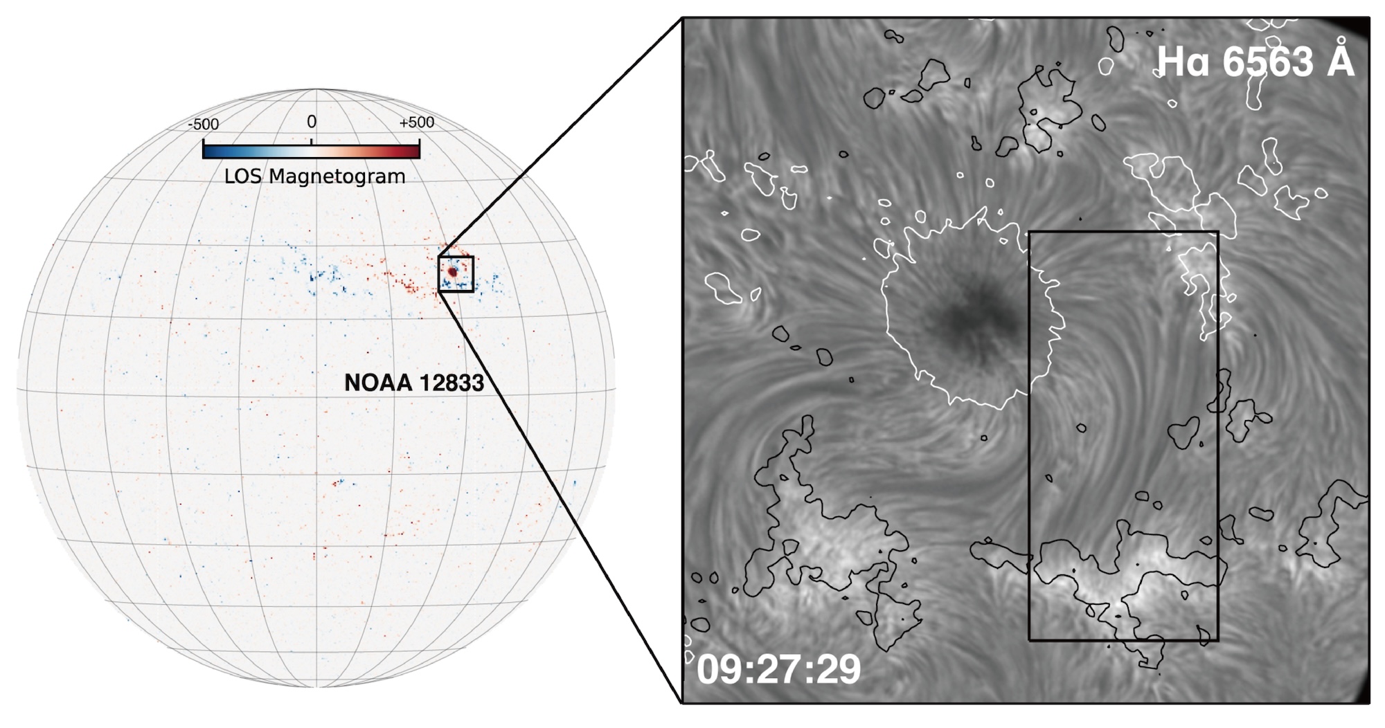
Location of the sunspot featured in this study, plus a closeup of the strands of plasma around the sunspot. Click to enlarge. [Adapted from Chen et al. 2025]

The images show a bundle of narrow strands of plasma stretching about 17,000–22,000 miles (28,000–36,000 kilometers). These plasma threads trace magnetic field lines as they emerge from the sunspot before diving down again in a network region, where the magnetic field is slightly enhanced at the border of a giant convective cell.

Driven by Reconnection

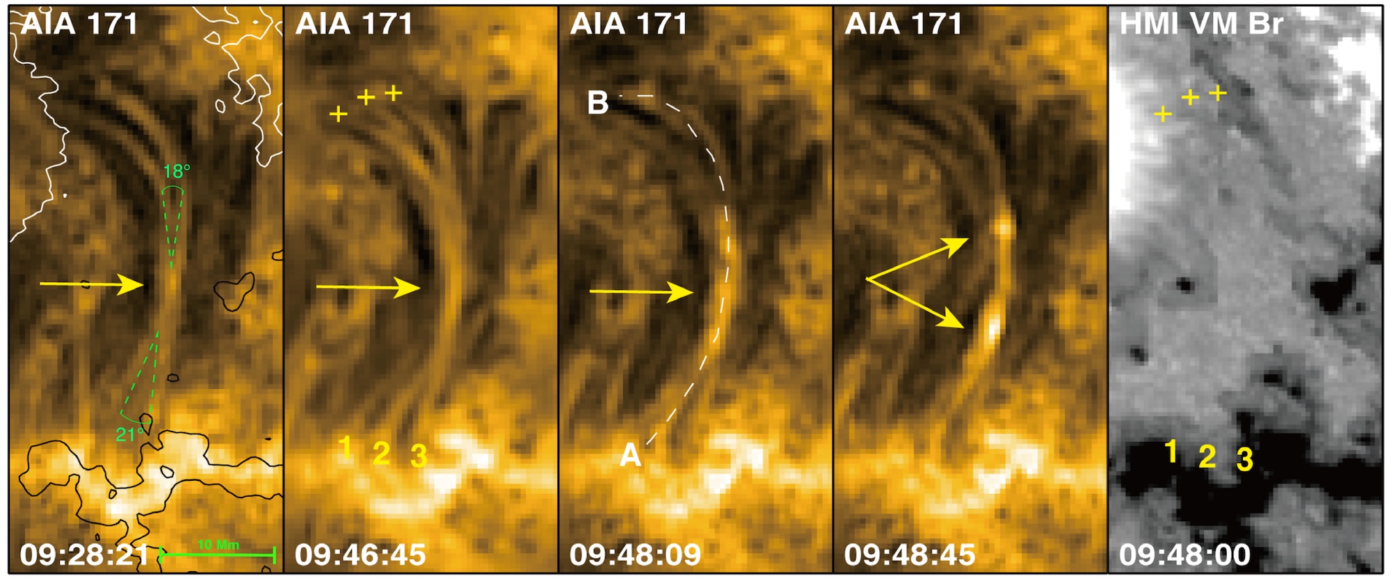
The plasma threads appear to lie nearly parallel to one another at the beginning of the observation. Images from all three facilities showed the plasma threads intertwining, providing evidence for the twisting of magnetic field lines predicted to happen when their footprints move around. (As further evidence for this footprint motion, the team also observed complicated flow patterns near one of the footprints.) This intertwining was followed by a sudden brightening where the threads were most tightly knotted, creating two bright β€œblobs” that traveled outward toward the footprints. Afterward, the threads resumed their nearly parallel state.

braiding magnetic field structures on the Sun

Images from Solar Dynamics Observatory. The first four images show the Sun at a wavelength of 17.1 nanometers, and the final image shows the radial magnetic field. The arrows indicate the location of the magnetic field braiding and the plasma β€œblobs.” Click to enlarge. [Adapted from Chen et al. 2025]

The team witnessed these bright points form and travel outward repeatedly, moving with projected velocities of 20–230 km/s. They posited that the motion and heating of these blobs of plasma was driven by the release of magnetic tension, and that the threads returned to a parallel configuration once reconnection was complete. They estimated that each of these events produced 1017 Joules, roughly the energy expected for small-scale reconnection events.

This work beautifully illustrates the process of magnetic reconnection on the Sun, showing how random motions can set the stage for the buildup of magnetic tension. The heating and acceleration of plasma that follows demonstrates how small-scale reconnection events like the ones shown here can provide the energy needed to heat the solar corona.

Citation

β€œWitnessing Magnetic Reconnection in Tangled Superpenumbral Fibrils Around a Sunspot,” Hechao Chen et al 2025 ApJ 995 94. doi:10.3847/1538-4357/ae12e9

The post Astronomers See Braided Magnetic Fields Above a Sunspot appeared first on AAS Nova.

When Winds Collide: Predicting the Effects of Stream Interaction Regions

14 January 2026 at 17:00

Illustration of the solar wind interacting with Earth's magnetic field

What happens when pileups of solar wind plasma collide with Earth’s protective magnetosphere? New work uses machine learning to examine how strongly these events affect our planet’s magnetic field.

Plasma Pileups

photograph of a coronal mass ejection

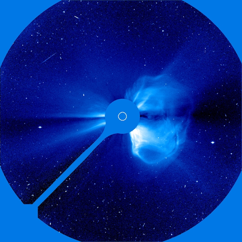
The Solar & Heliospheric Observatory (SOHO) took this coronagraphic image of a coronal mass ejection on 20 April 1998. [SOHO (ESA & NASA)]

Geomagnetic storms driven by solar activity paint night skies with glowing aurorae, but they also threaten spacecraft electronics with showers of high-energy particles. While immense eruptions of solar plasma and magnetic fields called coronal mass ejections are the most infamous example of solar activity, a team led by Yudong Ye (Sun Yat-Sen University) recently focused on another, less destructive form of activity: stream interaction regions.

Stream interaction regions arise when slow-moving solar wind is struck from behind by faster-moving solar wind emitted later. The collision of the two solar wind streams creates a tangle of compressed plasma and strong magnetic fields capable of peeling back Earth’s protective magnetosphere and dumping in high-energy charged particles, with beautiful yet harmful results.

Machine Learning Method

Though stream interaction regions are less disruptive than coronal mass ejections, they’re far more common; they frequently needle Earth’s magnetosphere, especially during the calmer years of the Sun’s activity cycle. Predicting how strongly a stream interaction region will influence Earth’s magnetosphere β€” in other words, how geoeffective it isΒ β€” is challenging, however. When two streams of solar wind collide, their properties combine in complex and nonlinear ways that traditional statistical investigations have struggled to pin down.

Now, Ye and collaborators have used machine learning to study the properties and impact of stream interaction regions in a physically meaningful way. They performed their study on a sample of 879 stream interaction events for which there is abundant information, such as temperature, magnetic field strength and direction, and solar wind conditions before and after the event.

illustration of the support vector machine framework

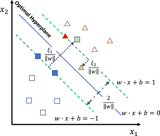
Illustration of the authors’ support vector machine framework. The optimal hyperplane is the boundary that best divides the data by maximizing the distance between the boundary and the data points nearest to it; these points are called support vectors. Square and triangle symbols represent two classes of data. Click to enlarge. [Ye et al. 2025]

Ye’s team based their framework on a support vector machine classifier: a classical machine learning algorithm that draws a mathematical boundary between groups of data while maximizing the distance between the boundary and the data points nearest to the dividing line. The support vector machine algorithm is well-suited to the task of modeling the geoeffectiveness of stream interaction regions because it doesn’t require a particularly vast dataset, can tolerate misclassified events, and allows for a physical interpretation of the results.

A Physical Interpretation

The team first reined in the model’s complexity by identifying the most important features in the dataset. They then determined which features or combination of features had the largest contribution to the output β€” in other words, which physical parameters most strongly determined the geoeffectiveness of the event.

illustration of magnetic reconnection in Earth's magnetosphere

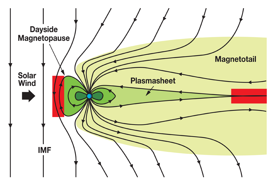
Illustration of how the interplanetary magnetic field (IMF) interacts with Earth’s magnetosphere. When the IMF points southward, as it does in this diagram, the impact on Earth’s magnetosphere is increased, with magnetic reconnection occurring in the red areas. Click to enlarge. [NASA]

Ye and collaborators found that the strongest determinants of an event’s geoeffectiveness were how long the solar wind was directed southward, the strength of the solar wind electric field, and the average and minimum strengths of the southward-pointing solar wind magnetic field. These results align with the current understanding of how energy is transferred from the solar wind to Earth’s magnetosphere through magnetic reconnection, a release of magnetic energy driven by rearrangement of magnetic fields. This shows how classical machine learning methods can enhance our ability to predict the outcome of oncoming space weather while simultaneously examining the physical drivers of the event.

Citation

β€œAssessing the Geoeffectiveness of Stream Interaction Regions Through Physically Interpretable Machine Learning,” Yudong Ye et al 2025 ApJ 993 10. doi:10.3847/1538-4357/ae0454

The post When Winds Collide: Predicting the Effects of Stream Interaction Regions appeared first on AAS Nova.

Selections from 2025: The Sun Changed Course in 2008

18 December 2025 at 17:00

extreme-ultraviolet image of the Sun

Editor’s Note: For the remainder of 2025, we’ll be looking at a few selections that we haven’t yet discussed on AAS Nova from among the most-downloaded articles published in AAS journals this year. The usual posting schedule will resume January 2nd.

The Sun Reversed Its Decades-Long Weakening Trend in 2008

Published September 2025

Main takeaway:

plots of solar wind parameters from 2008 to 2025

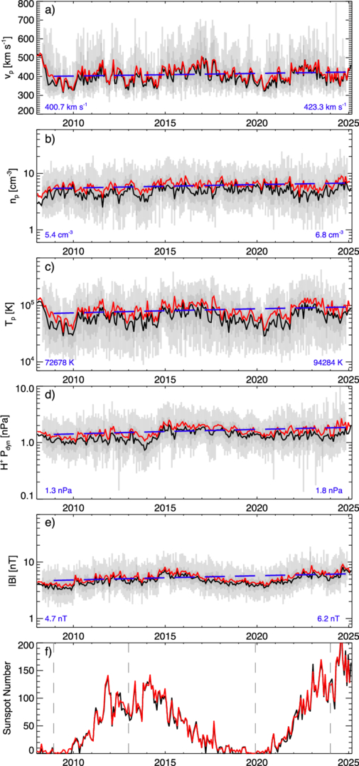
Various solar wind parameters measured at Earth’s orbital distance from 2008 to 2025. [Jasinski and Velli 2025]

Jamie Jasinski (NASA’s Jet Propulsion Laboratory) and Marco Velli (NASA’s Jet Propulsion Laboratory and the University of California, Los Angeles) analyzed solar wind data from 2008 to 2025 and found that many solar wind parameters such as speed, density, temperature, and magnetic field strength increased over that time period. This increase ran counter to expectations that the Sun may be entering a historically low period of activity in 2008.

Why it’s interesting:

The Sun undergoes an 11-year activity cycle that is driven by a change in its internal magnetic field structure. As the Sun’s magnetic activity changes, the number of sunspots, the frequency of solar flares and coronal mass ejections, and the intensity of the solar wind vary as well. Atop these mostly regular 11-year changes are longer-term variations. A recent example of this longer-term behavior began in the 1980s, when an overall weakening trend was stamped upon the usual 11-year cycle. This decline led to an exceptionally deep solar minimum in 2008, leading researchers to suspect that the Sun’s activity level might remain low for decades.

The historical context for a prolonged weak period:

Though the Sun reversed its weakening activity trend in 2008, a prolonged period with little solar activity wouldn’t have been unprecedented. Astronomers have monitored and counted sunspots for centuries, allowing modern-day researchers to investigate the Sun’s behavior long before spacecraft began to study our home star. In the historical record, there are two instances of weak solar activity spanning multiple decades: the Maunder minimum in 1645–1715 and the Dalton minimum in 1790–1830. Compared to the 11-year solar cycle, these longer-term behaviors are more difficult to predict, and their causes are uncertain.

Citation

Jamie M. Jasinski and Marco Velli 2025 ApJL 990 L55. doi:10.3847/2041-8213/adf3a6

The post Selections from 2025: The Sun Changed Course in 2008 appeared first on AAS Nova.

How Solar Flares Hint That They’re About to Happen

1 December 2025 at 17:00

Images of a solar flare at different wavelengths

Forecasting solar flares is one of the major challenges facing solar physicists today. New research finds that non-thermal emission can precede a solar flare by more than an hour, and this early emission may signal whether the flare will be accompanied by an explosion of plasma.

Flare Flavors

photograph of a coronal mass ejection

The Solar & Heliospheric Observatory (SOHO) took this coronagraphic image of a coronal mass ejection on 20 April 1998. [SOHO (ESA & NASA)]

Solar flares come in two basic flavors: eruptive and confined. EruptiveΒ flares are accompanied by the launch of tangled clouds of plasma and magnetic fields called coronal mass ejections.Β Confined flares, so called because the solar plasma remains confined to the Sun, feature only a brief blast of high-energy radiation.

Both solar flares and coronal mass ejections can disrupt everyday life on Earth, with flares knocking out radio communications and coronal mass ejections threatening spacecraft electronics and power grids. Given these real-life risks, as well as the potential for probing the physics behind the activity on the Sun and other stars, it’s critical to be able to identify signs of upcoming flares.

Looking at the Lead-Up

Luckily, there’s growing evidence that the Sun sends out subtle signals that a flare is soon to happen. One early sign of an impending flare is an increase in the non-thermal velocity of the plasma at the flare’s location. This phenomenon has been spotted in individual flares, but it hasn’t been studied and characterized for a large sample of flares β€” until now.

example of increasing non-thermal velocity before a solar flare

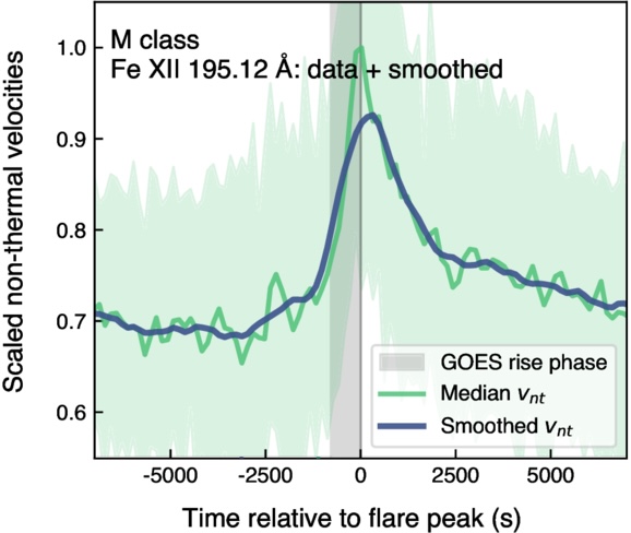
Demonstration of the increase in non-thermal velocity seen in an M-class flare compared to the onset and rise time of the soft X-ray flux (gray shaded area). [Adapted from To et al. 2025]

A recent research article led by Andy S. H. To (European Space Agency) takes the first systematic, large-scale approach to studying the non-thermal velocity changes that precede solar flares. The team amassed a sample of 1,449 solar flares that were seen by the Hinode spacecraft, the Geostationary Operational Environmental Satellite (GOES), and the Solar Dynamics Observatory (SDO). Hinode provided the spectral information needed to identify increases in the non-thermal velocity, GOES provided the flare start times, and SDO provided detailed information on the location and appearance of each flare.

Of the flares in the sample, 83% were moderately powerful C-class flares, 18% were stronger M-class flares, and 1% were the most powerful X-class flares. To’s team identified a clear trend across all types of flares: the non-thermal velocity increases 4–25 minutes before the flare’s X-ray emission begins to rise, peaks when the X-ray emission peaks, and decays as the flare decays. The team found some evidence that for smaller flares, the velocity increase begins in spectral lines that trace cooler plasma before spreading to lines probing hotter plasma, but more work is needed to confirm this trend.

More Details

Examples of flares with and without coronal mass ejections

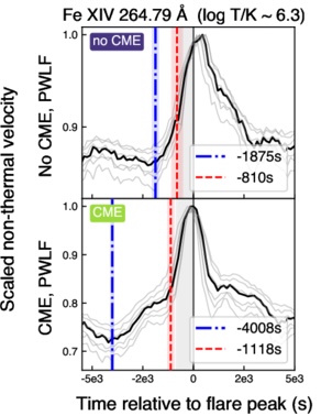
Examples of flares with and without coronal mass ejections. [Adapted from To et al. 2025]

Certain flares give even earlier hints of upcoming activity. M-class flares and some C-class flares exhibit what To’s team calls β€œprecursor emission,” which emerges roughly 30–60 minutes before the flare’s X-ray emission peaks. The team also identified differences in precursor emission between confined and eruptive flares: eruptive flares display precursor emission over a broad range of spectral lines starting 45–74 minutes before the flare peaks, while confined flares show precursor emission later (31–54 minutes before peak) and in only a few spectral lines.

These results suggest that changes in the non-thermal velocity of solar plasma can not only signal when and where a flare is likely to arise, but also whether the flare will be accompanied by a potentially destructive coronal mass ejection. Upcoming missions like the Multi-slit Solar Explorer and SOLAR-C will give an even better view of the early stages of solar flares, helping to illuminate the physics behind them and enhancing our ability to forecast them.

Citation

β€œSystematic Nonthermal Velocity Increase Preceding Soft X-Ray Flare Onset: A Large-Scale Hinode/EIS Study,” Andy S. H. To et al 2025 ApJ 993 102. doi:10.3847/1538-4357/ae07de

The post How Solar Flares Hint That They’re About to Happen appeared first on AAS Nova.
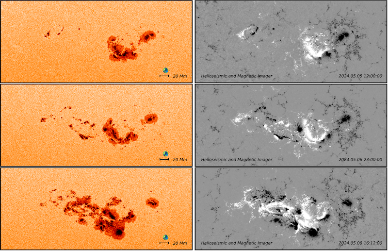
Featured Image: Mother’s Day Superstorms

28 July 2025 at 17:00

closeup of a solar active region

solar active regions

Evolution of a cluster of active regions as seen in continuum emission (left column) and radial magnetic field (right column). Click to enlarge. [Dikpati et al. 2025]

Around Mother’s Day (12 May) last year, the Sun put on a spectacular display of solar activity. A clash between solar active regions incited 14 coronal mass ejections, launched multiple high-energy X-class solar flares, and sent shimmering aurorae as far south as Florida. The images above and to the right show the source of all this excitement: the active regions AR 13664 and AR 13668. In a recent research article, Mausumi Dikpati (High Altitude Observatory) and coauthors examined the origins of this cluster of active regions and why they were such a powerful source of solar storms. Their investigation showed that there are certain regions on the Sun where solar storms are more likely to arise. These regions occur where the Sun’s undulating bands of magnetic activity draw farthest apart, preventing oppositely directed magnetic fields from canceling one another out. In the case of the Mother’s Day superstorms, active regions 13664 and 13668 developed on the heels of a decaying active region, further contributing to their magnetic complexity. Ultimately, this analysis suggested that it may be possible to forecast damaging solar activity weeks in advance by predicting the locations of magnetically complex active regions and following their evolution. To learn more about the active regions that gave rise to the Mother’s Day superstorms, be sure to check out the full article linked below.

Citation

β€œMother’s Day Superstorms: Pre- and Post-Storm Evolutionary Patterns of ARs 13664/8,” Mausumi Dikpati et al 2025 ApJ 988 108. doi:10.3847/1538-4357/addd09

The post Featured Image: Mother’s Day Superstorms appeared first on AAS Nova.
Minding the Gaps in Solar Wind Data

9 July 2025 at 17:00

solar wind

Spacecraft scattered throughout the solar system keep tabs on the solar wind, but the measurements are dotted with data gaps. How can scientists prevent these gaps from biasing their studies of the solar wind?

Sampling the Solar Wind

intracluster medium

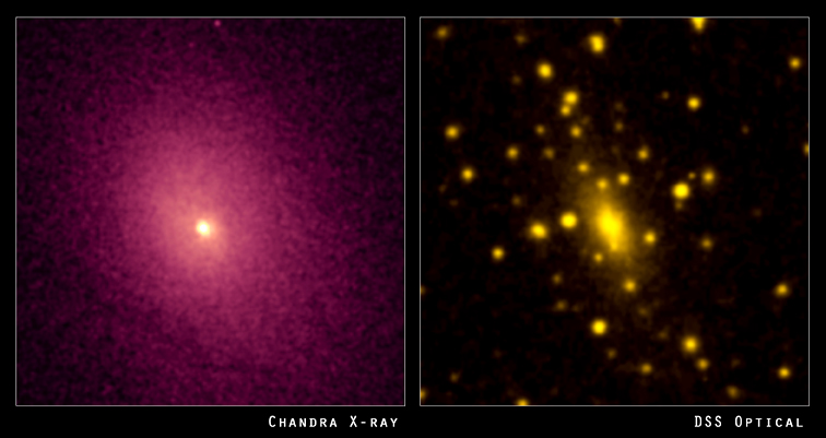
Left: the distribution of hot gas between the galaxies in the cluster Abell 2029. Right: the visible light from the galaxies in the cluster. [X-ray: NASA/CXC/UCI/A.Lewis et al. Optical: Pal.Obs. DSS]

The solar wind is a tenuous, fast-moving, turbulent plasma that constantly streams out from the Sun. Studying the solar wind is important for understanding how potentially damaging space weather events like coronal mass ejections travel through the solar system. Solar wind studies also have far-reaching implications, since solar-wind-like plasmas exist throughout the universe, such as in the sparse medium between galaxies in a cluster.

Luckily, there are many spacecraft that sample the solar wind from various locations within our solar system. Unluckily, many of these spacecraft do not continuously monitor the solar wind. For example, when a spacecraft orbiting a planet dips into the planet’s atmosphere, this detour creates an hours-long gap in solar wind monitoring.

The Impact of Data Gaps

How do these data gaps affect studies of the solar wind? In a recent research article, Daniel Wrench and Tulasi Parashar (Victoria University of Wellington) approached this question in terms of how gaps affect the structure function:Β a mathematical description of how the solar wind fluctuates over different length or time scales.

Wrench and Parashar introduced random artificial gaps into data from the Parker Solar Probe, which monitors the solar wind continuously, and compared the structure functions calculated from the continuous and interrupted data sets. They used the difference between the true structure function β€” calculated from the continuous data set β€” and the structure functions from the artificially gapped data sets to develop a correction factor.

bar plot of correction method performance

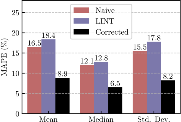
Performance of the correction factor method (black) compared to the uncorrected, gapped data (red) or gaps filled using linear interpolation (blue). MAPE is the mean absolute percentage error. [Wrench & Parashar 2025]

The team then tested their correction factor using data from the Wind spacecraft, which continuously monitors the solar wind from the L1 Lagrange point. The team calculated the structure function from 1) the continuous data set, 2) the artificially gapped data, 3) the gapped data with linear interpolation used to fill the gaps, and 4) the gapped data with the correction factor applied. This test showed that the correction factor performs better than other commonly used gap-handling methods, such as linear interpolation, which can systematically underestimate the structure function. Using the correction factor, the error in the structure function remained below 50% even when 95% of the data were missing.
plot of structure function from Voyager 1 data

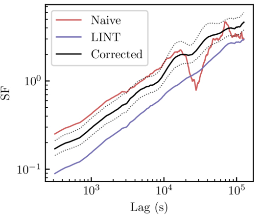
Structure function calculated from uncorrected Voyager 1 data (red), linearly interpolated data (blue), and corrected data (black). Both the linear interpolation method and the correction factor method remove the artifact around a lag of 3Γ—104 seconds, but the correction factor method does not suppress the signal like the linear interpolation method does. [Adapted from Wrench & Parashar 2025]

Correcting Voyager 1

Finally, the authors applied their validated method to data from Voyager 1. Data from the two Voyager spacecraft are extremely scientifically valuable β€” no other spacecraft have ventured as far from the Sun and can measure the solar wind at such large distances. The data are also extremely sparse; one segment used in this work was missing 85% of the data. This means that an effective method of correcting these data has potentially huge scientific significance.

Wrench and Parashar applied their correction factor to the Voyager 1 data, showing that this method handily removes artifacts while avoiding the underestimation introduced by linear interpolation. While the authors saved the interpretation of the newly corrected Voyager 1 data for future research, this study makes it clear that even large data gaps needn’t hinder studies of the solar wind.

Citation

β€œDebiasing Structure Function Estimates from Sparse Time Series of the Solar Wind: A Data-Driven Approach,” Daniel Wrench and Tulasi N. Parashar 2025 ApJ 987 28. doi:10.3847/1538-4357/addc6a

The post Minding the Gaps in Solar Wind Data appeared first on AAS Nova.
Understanding Chemtrails and Geoengineering

17 February 2025 at 05:43
Chemtrails are real enough. Government agencies have been spraying the atmosphere with aerosols for decades. Solar Radiation Modification techniques, particularly Stratospheric Aerosol Injection, are intended to combat global warming but the potential agricultural and ecological damage is very concerning. I relate these developments to biblical prophecies about apocalyptic events.

The Physics of Creation | Day 4

18 January 2025 at 03:14
Day 4 of creation, God made the Sun, Moon, planets, and stars, establishing them as luminaries in the heavens. The language of the Bible uses an Earth-observer perspective, meaning that light from celestial bodies was instantly visible. Additionally, I confront naturalistic explanations for celestial origins, proposing a creationist model.

If Jupiter Disappeared Would Earth Face More Asteroid Hits?

27 February 2026 at 13:56

Jupiter dominates the Solar System’s architecture. At about 318 times Earth’s mass and orbiting far beyond Mars, it acts as a gravitational gatekeeper, tugging on asteroids and comets that might otherwise stay put or never reach the inner planets. Remove Jupiter from the picture and Earth’s impact environment would change in complicated ways. It would […]

The post If Jupiter Disappeared Would Earth Face More Asteroid Hits? appeared first on Curiosmos.

Crowds Flood New York City Streets for First Day of Manhattanhenge

29 May 2026 at 16:12
People filled the streets of New York on Thursday to get a glimpse of this year’s first Manhattanhenge. The spectacular view of the sun setting, flanked by the city’s streetscapes, will also occur on Friday and July 11 and 12.

Do we know how long it took the Sun to form?

19 November 2024 at 00:03

While there is consensus that our Sun formed about 4.6 billion years ago from a molecular cloud of gas and dust, less has been known about how long the formation of the star...

The post Do we know how long it took the Sun to form? first appeared on Science Illustrated.

❌