❌

Normal view

Britain’s Power Grid Has a Blind Spot for Extreme Solar Storms, New Research Reveals

30 July 2026 at 19:13

In May 2024, the strongest geomagnetic storm in two decades pushed the Northern Lights far enough south to become visible across much of the UK and beyond. Now, a study that appeared in Royal Society Open Science reveals that the incident also exposed important gaps in how the UK monitors and prepares its power grid, satellites, and aviation for future extreme space weather.

The storm reached a G5 rating, which is the highest level on the geomagnetic storm scale used by NOAA, as a result of five coronal mass ejections reaching Earth within a period of two days. Researchers with the Space Environment Impacts Expert Group (SEIEG) stated that although the storm caused only relatively minor disruption, it revealed shortcomings in the UK’s capacity to monitor and prepare for more severe space weather events.

The SEIEG then made 14 recommendations to the UK government addressing matters such as grid monitoring, satellite operations, and space weather forecasting. Richard Horne, chair of SEIEG and head of space weather at the British Antarctic Survey, recently gave a presentation on the findings at the Royal Astronomical Society’s National Astronomy Meeting in Birmingham.

A Storm That Tested the Limits

Researchers estimate that the May 2024 storm was a one-in-13-year event. By contrast, a Carrington-class storm, like the 1859 event that defines the standard for extreme space weather, has about a 1% chance of occurring in any given year. This means that a much more disruptive storm is still possible. The SEIEG report uses the 2024 storm as a practical example to assess how prepared the UK is for a more severe event.

“The Northern Lights were the most visible sign of the May 2024 storm, but they were only one part of a much broader space weather event that tested the UK’s critical infrastructure. The storm highlighted where we need better monitoring, better forecasting and more research so we’re prepared for a more severe event in the future,” Horne said.

The Blind Spot in Britain’s Power Grid

Geomagnetic storms create electric fields at Earth’s surface that can drive geomagnetically induced currents (GICs) through long conductive systems, including power transmission networks. High levels of GICs can overheat transformers, disrupt their normal function, and in severe cases cause damage that may lead to failures across parts of the power grid.

Currently, there are no GIC monitors in operation in England or Wales. The SEIEG report recommends establishing a network of monitors to assess how much current various transformer designs can tolerate before sustaining damage.

New Zealand as the Model

The report cites New Zealand as an example of effective monitoring. Since it is at a similar geomagnetic latitude, the country faces similar space weather risks, and its grid operators monitor around 93 transformers across 28 substations. Unlike in England and Wales, where monitoring is absent, these operators have verified their models using actual measurements and implemented operational mitigation procedures during the May 2024 storm.

Crowded Skies, Rising Risk

The storm also affected satellites in orbit. Almost 5,000 satellites adjusted their orbits during the storm. Satellites licensed in the UK saw their number of collision warnings rise by 35%. Since there are now so many objects in low-Earth orbit, a serious storm could raise the risk of collisions, possibly resulting in debris and causing additional incidents.

Preparing for Future Storms

SEIEG also recommends improving forecasts of coronal mass ejections and solar energetic particle events to provide two to three hours of warning before severe geomagnetic storms reach Earth. Improved forecasts could allow grid operators, satellite controllers, and airlines to take protective measures before severe geomagnetic storms arrive. 

“One of the biggest lessons from the May 2024 storm is that we still have important gaps in our monitoring and understanding of how severe space weather could affect UK infrastructure,” said Horne. “We were fortunate that this was not a one-in-100-year event. We now have an opportunity to strengthen our monitoring, improve our forecasts and make sure the UK is better prepared before a much larger storm occurs.”

The 14 recommendations are now under review by the UK government. Whether these steps will be taken before a Carrington-scale storm occurs remains uncertain. With this extreme class of storms remaining a realistic possibility, the researchers argue that improving monitoring and forecasting now could reduce the impact of a future extreme event.

Austin Burgess is a writer and researcher with a background in sales, marketing, and data analytics. He holds an MBA, a Bachelor of Science in Business Administration, and a data analytics certification. His work focuses on breaking scientific developments, with an emphasis on emerging biology, cognitive neuroscience, and archaeological discoveries.

Monthly Roundup: Science of the Sun

27 April 2026 at 17:00

three images of the Sun

The Sun’s activity history, the sources of tiny jets, and how magnetic fields might impact space weather forecasts: today’s Monthly Roundup introduces a trio of recent research articles from the Astrophysical Journal that tackle hot topics in solar physics.

From 1755 to 2020: Reconstructing Centuries of Solar Activity

Since the 1970s, regular monitoring of the Sun’s magnetic field has allowed researchers to decipher the Sun’s behavior as it cycles through periods of low and high activity. But what resources exist for studying the Sun’s past behavior? To investigate the long-term behavior of the Sun, researchers reach for historical records of sunspots, which stretch back to the 1700s.

maps of simulated photospheric magnetic fields

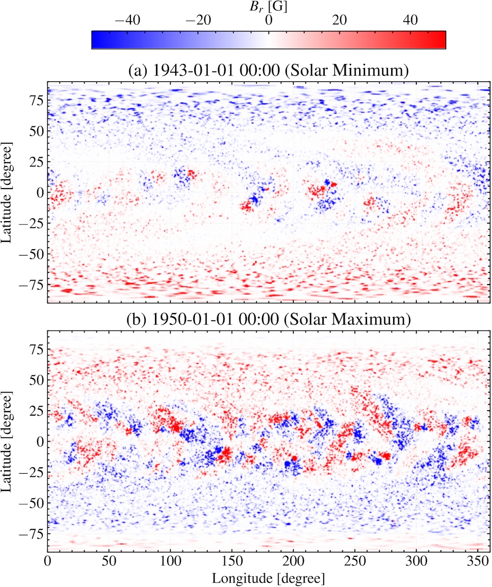
Example maps of the simulated photospheric radial magnetic field during a period of low (top) and high (bottom) solar activity. Click to enlarge. [Jha et al. 2026]

Bibhuti Kumar Jha (Southwest Research Institute) and collaborators explored whether historical records and modern statistics could be used to reconstruct the behavior of the solar magnetic field centuries into the past. Jha’s team used recorded sunspot numbers from 1755 to 2020 as an input for their newly developed Synthetic Active Region Generator, which generates synthetic solar active regions based on known statistics of these regions. This catalog of active regions becomes the input for the Advective Flux Transport model, which simulates the active regions as they emerge and evolve, allowing for an estimation of the magnetic field across the Sun’s disk.

Jha and coauthors found that this method successfully reproduced the expected large-scale behavior of the Sun’s magnetic field across multiple solar cycles, such as the reversal of the polarity of the solar magnetic field near the peak of the activity cycle. While this work highlights the impressive results obtained from combining historical sunspot records with modern sunspot statistics, the team pointed out that this method cannot accurately reproduce all quantities because of the nonlinear nature of the underlying physics. Future work will refine the model further, and in the meantime, the team’s simulated historical magnetic field maps will be made publicly available.

Where Do the Tiniest Coronal Jets Come From?

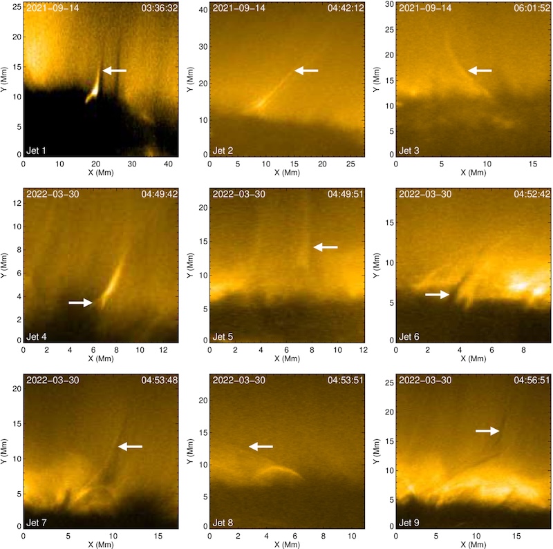
The Sun’s atmosphere is filled with an ever-shifting maze of magnetic field lines, which reconfigure and release pent-up magnetic energy in a process called magnetic reconnection. Magnetic reconnection can launch particles and heat plasma, and it’s thought to be responsible for driving jets on a variety of scales in the Sun’s tenuous outer atmosphere, or corona. Annu Bura (Indian Institute of Astrophysics; Pondicherry University) and coauthors investigated the physical origins of the smallest of these reconnection driven jets, picoflare jets, using data from the Extreme Ultraviolet Imager on board Solar Orbiter. Solar Orbiter has ventured within 0.3 au of the Sun, and its Extreme Ultraviolet Imager has returned exceptionally precise high-energy images of our home star.

Examples of coronal jetlets

Examples of jets identified in this study. You can see an animation of this figure. [Bura et al. 2026]

Bura and collaborators identified picoflare jets by the presence of a hot, bright spire coupled with a cool, dark streak, forming a structure shaped like the letter “Y” upside down. They found that the bright and dark features were on average 650 and 490 kilometers wide, respectively, with a typical jet length of 16,900 kilometers. They also found that the bright features moved more quickly than the dark features, and the jets tended to last about 6 minutes. Overall, these measurements place the jets in between the scales expected for picoflare jets and slightly larger features called jetlets, though the energies are consistent with expectations for picoflare jets.

Using radiation magnetohydrodynamics simulations, the team explored the origins of their sample of jets. The simulations suggested that the bright features arose from hot, tenuous coronal plasma, while the accompanying dark features were due to cooler, denser plasma venturing upward from deeper in the Sun’s atmosphere, in the chromosphere. Overall, the simulations and observations support a picture in which picoflare-scale jets are driven by magnetic reconnection after magnetic flux emerges through the Sun’s surface. This echoes the formation route of larger coronal jets, suggesting that this process may apply to a wide range of physical scales.

Investigating the Influence of the Solar Polar Magnetic Field

The vast majority of our observations of the Sun have come from within a few degrees of the ecliptic plane, either from telescopes situated on Earth’s surface or from spacecraft that stuck close to the plane of our solar system. With rare but notable exceptions — the Ulysses spacecraft, which measured the Sun’s magnetic field and plasma environment from a near-polar orbit, and Solar Orbiter, which took the first-ever image of the Sun’s poles in November 2025 — the Sun’s poles have remained hidden from our instruments.

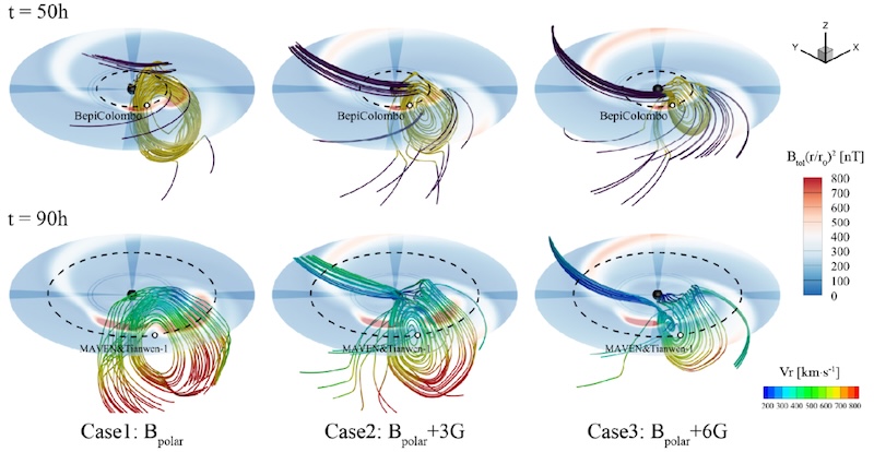
Our limited knowledge of the Sun’s polar magnetic field has consequences for our ability to model space weather events like coronal mass ejections. A team led by Xiao Zhang (Chinese Academy of Sciences; University of Chinese Academy of Sciences) has used numerical simulations to investigate how solar polar magnetic field conditions influence the propagation of a coronal mass ejection (CME) through the solar system.

Simulation results showing the propagation and expansion of a coronal mass ejection

Simulation results showing how the propagation and expansion of a CME are affected by the polar magnetic field strength. Click to enlarge. [Zhang et al. 2026]

The team simulated a CME from 4 December 2021, which was observed by the BepiColombo spacecraft at Mercury and Tianwen-1 and MAVEN at Mars. The simulations showed that as the polar magnetic field strength increases, the CME’s movement through the solar system becomes slower. CMEs typically expand as they billow outward from the solar corona and sweep past the planets; increasing the polar magnetic field strength slowed the CME’s expansion as well. A stronger polar magnetic field also alters the background solar wind, making it slower and denser. Overall, these results demonstrate that the strength of the Sun’s poorly constrained polar magnetic field can have a significant impact on the movement and evolution of a CME. In future work, Zhang’s team plans to expand their investigation to a larger sample of CMEs.

Citation

“Historical Reconstruction of Solar Surface Magnetism from Cycles 1–24 Using the Synthetic Active Region Generator and the Advective Flux Transport Model,” Bibhuti Kumar Jha et al 2026 ApJ 997 279. doi:10.3847/1538-4357/ae279a

“On the Origin of Coronal Picoflare Jets,” Annu Bura et al 2026 ApJ 1000 94. doi:10.3847/1538-4357/ae48e6

“Influence of Solar Polar Magnetic Fields on the Propagation of Coronal Mass Ejections,” Xiao Zhang et al 2026 ApJ 1000 200. doi:10.3847/1538-4357/ae4c54

The post Monthly Roundup: Science of the Sun appeared first on AAS Nova.

Comets Are Lizards: Watching C/2023 P1 Regrow Its Tail

13 April 2026 at 17:00

comet C/2023 P1

Researchers tracked the tail of comet C/2023 P1 (Nishimura) as it interacted with a string of coronal mass ejections, leading to the first-ever quantitative analysis of a cometary tail detachment event.

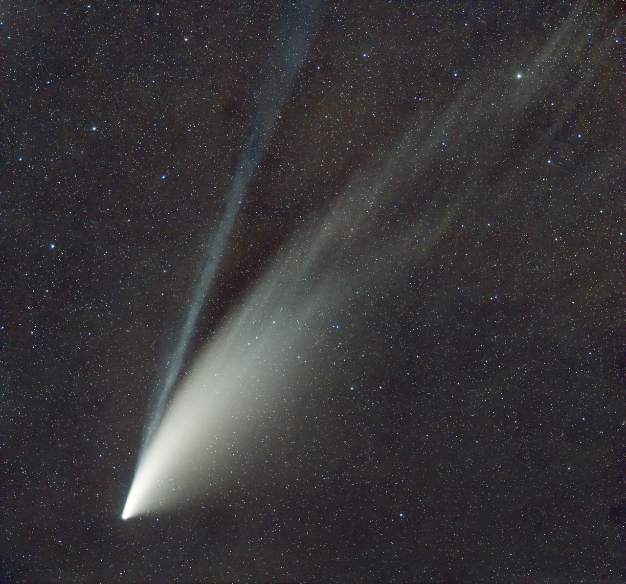
C/2020 F3 (NEOWISE)

A photo of comet C/2020 F3 (NEOWISE) showing its narrow bluish ion tail and broader white dust tail. [Juan lacruz; CC BY-SA 4.0]

A Comet’s Journey

When comets journey into the inner solar system, they tend to do so sporting two tails: a dust tail that sweeps back from the comet along its curved trajectory and an ion tail that points away from the Sun, in the direction of the interplanetary magnetic field.

The ion tail, which forms when ultraviolet light from the Sun ionizes gas in a comet’s fuzzy coma, interacts with structures in the solar wind, causing it to shift, sputter, and sometimes even disconnect entirely. Now, for the first time, researchers have quantified the timescales involved when a comet loses — and regrows — its tail.

The Tale of a Tail

Shaheda Begum Shaik (George Mason University; US Naval Research Laboratory) and collaborators studied this phenomenon in observations of the comet C/2023 P1 (Nishimura) from 1 to 14 September 2023. In high-resolution images from the Solar Orbiter Heliospheric Imager, Shaik’s team analyzed the dynamics of C/2023 P1’s tail as the comet braved blustery solar wind conditions in the inner solar system.

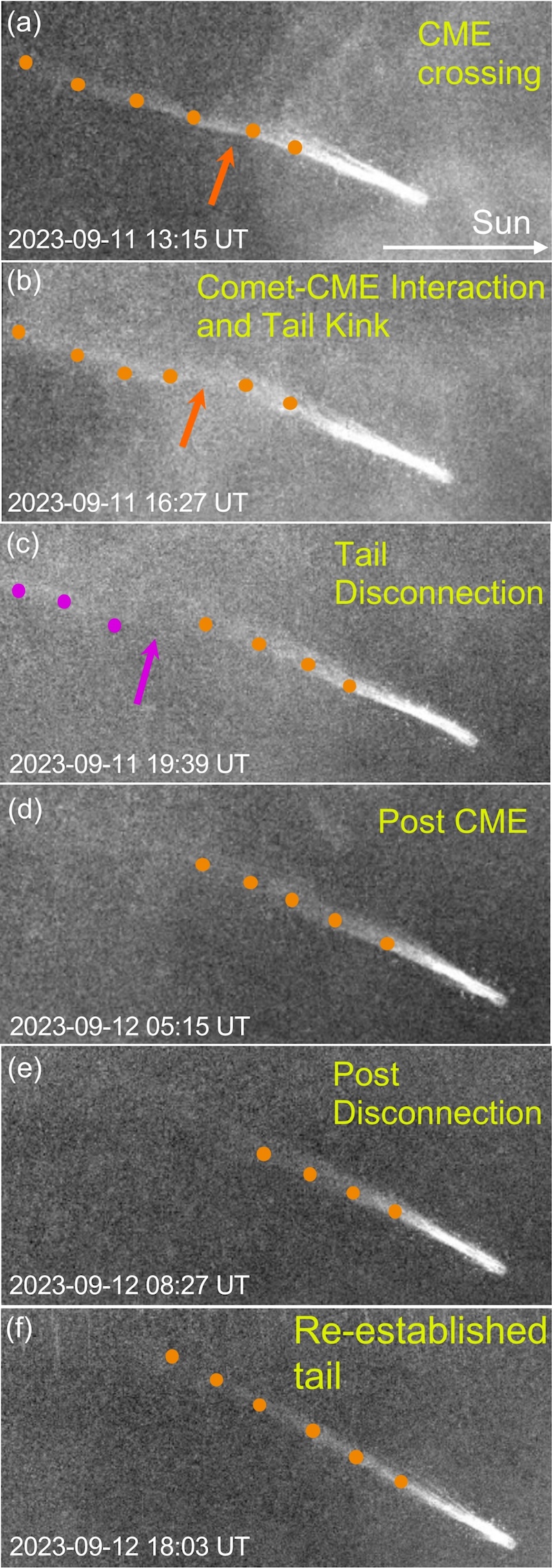
In a two-week period, the comet underwent four separate tail disconnection events, in which the connection between the ion tail and the comet was severed. Each of these events coincided with the passage of a coronal mass ejection: a tangled mass of solar plasma and magnetic fields ejected from the Sun’s outer atmosphere.

tail disconnection event observations

Solar Orbiter Heliospheric Imager observations of the 11 September 2023 tail disconnection event, which was driven by a passing coronal mass ejection (CME). [Shaik et al. 2026]

Lizard-Like Regrowth

Focusing on the tail disconnection event with the highest-resolution and highest-cadence data, Shaik’s team observed constant small-scale fluttering of the ion tail, reflecting the buffeting of the tail by the solar wind. The tail then developed a kink, which the team speculated is due to compressed solar wind plasma piling up in front of an oncoming coronal mass ejection. The wide-field images show the coronal mass ejection advancing upon the comet and the comet’s tail seemingly being sliced in two.

The free-floating tail segment sped away from the comet at roughly 295 km/s, likely indicating that the tail became caught up in and was transported by the flank of the coronal mass ejection as it barreled past the comet. The timescale and geometry of the event suggest that the interaction of the coronal mass ejection’s magnetic field with the comet’s tail was responsible for the disconnection.

Over the following 24 hours, the comet’s tail slowly regrew at a rate of 86 km/s to its original length of 1.9 million kilometers. The rate of regrowth is likely determined by several factors, such as the rate at which the comet produces ions and the local magnetic field configuration. This work represents a first look at the quantitative behavior of a tail disconnection event, paving the way for future investigations of cometary behavior and a greater understanding of the complex magnetic and plasma environment of the inner solar system.

Citation

“The First Quantitative Study of Cometary Tail Regrowth Following a Coronal Mass Ejection-Driven Disconnection Event,” Shaheda Begum Shaik et al 2026 ApJ 999 60. doi:10.3847/1538-4357/ae3bdb

The post Comets Are Lizards: Watching C/2023 P1 Regrow Its Tail appeared first on AAS Nova.

When Winds Collide: Predicting the Effects of Stream Interaction Regions

14 January 2026 at 17:00

Illustration of the solar wind interacting with Earth's magnetic field

What happens when pileups of solar wind plasma collide with Earth’s protective magnetosphere? New work uses machine learning to examine how strongly these events affect our planet’s magnetic field.

Plasma Pileups

photograph of a coronal mass ejection

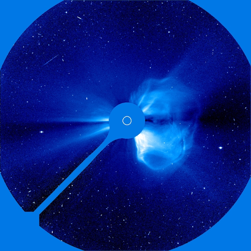
The Solar & Heliospheric Observatory (SOHO) took this coronagraphic image of a coronal mass ejection on 20 April 1998. [SOHO (ESA & NASA)]

Geomagnetic storms driven by solar activity paint night skies with glowing aurorae, but they also threaten spacecraft electronics with showers of high-energy particles. While immense eruptions of solar plasma and magnetic fields called coronal mass ejections are the most infamous example of solar activity, a team led by Yudong Ye (Sun Yat-Sen University) recently focused on another, less destructive form of activity: stream interaction regions.

Stream interaction regions arise when slow-moving solar wind is struck from behind by faster-moving solar wind emitted later. The collision of the two solar wind streams creates a tangle of compressed plasma and strong magnetic fields capable of peeling back Earth’s protective magnetosphere and dumping in high-energy charged particles, with beautiful yet harmful results.

Machine Learning Method

Though stream interaction regions are less disruptive than coronal mass ejections, they’re far more common; they frequently needle Earth’s magnetosphere, especially during the calmer years of the Sun’s activity cycle. Predicting how strongly a stream interaction region will influence Earth’s magnetosphere — in other words, how geoeffective it is — is challenging, however. When two streams of solar wind collide, their properties combine in complex and nonlinear ways that traditional statistical investigations have struggled to pin down.

Now, Ye and collaborators have used machine learning to study the properties and impact of stream interaction regions in a physically meaningful way. They performed their study on a sample of 879 stream interaction events for which there is abundant information, such as temperature, magnetic field strength and direction, and solar wind conditions before and after the event.

illustration of the support vector machine framework

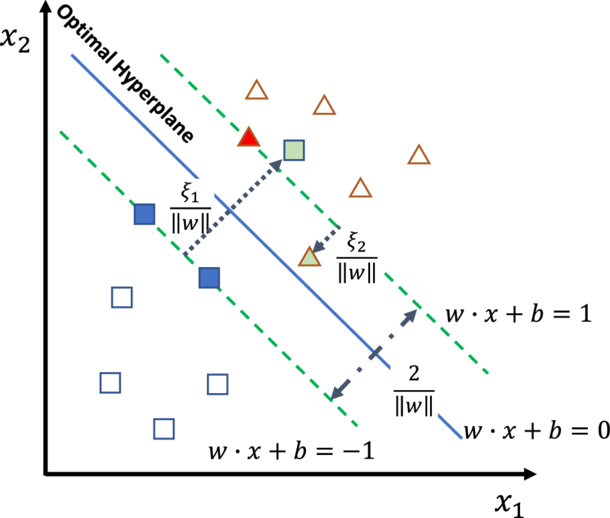
Illustration of the authors’ support vector machine framework. The optimal hyperplane is the boundary that best divides the data by maximizing the distance between the boundary and the data points nearest to it; these points are called support vectors. Square and triangle symbols represent two classes of data. Click to enlarge. [Ye et al. 2025]

Ye’s team based their framework on a support vector machine classifier: a classical machine learning algorithm that draws a mathematical boundary between groups of data while maximizing the distance between the boundary and the data points nearest to the dividing line. The support vector machine algorithm is well-suited to the task of modeling the geoeffectiveness of stream interaction regions because it doesn’t require a particularly vast dataset, can tolerate misclassified events, and allows for a physical interpretation of the results.

A Physical Interpretation

The team first reined in the model’s complexity by identifying the most important features in the dataset. They then determined which features or combination of features had the largest contribution to the output — in other words, which physical parameters most strongly determined the geoeffectiveness of the event.

illustration of magnetic reconnection in Earth's magnetosphere

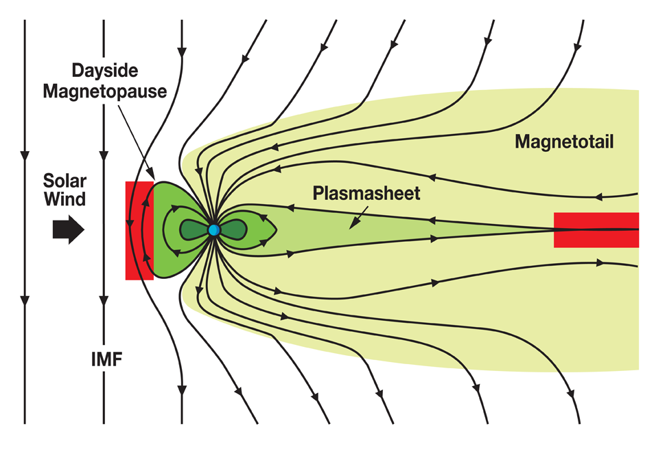
Illustration of how the interplanetary magnetic field (IMF) interacts with Earth’s magnetosphere. When the IMF points southward, as it does in this diagram, the impact on Earth’s magnetosphere is increased, with magnetic reconnection occurring in the red areas. Click to enlarge. [NASA]

Ye and collaborators found that the strongest determinants of an event’s geoeffectiveness were how long the solar wind was directed southward, the strength of the solar wind electric field, and the average and minimum strengths of the southward-pointing solar wind magnetic field. These results align with the current understanding of how energy is transferred from the solar wind to Earth’s magnetosphere through magnetic reconnection, a release of magnetic energy driven by rearrangement of magnetic fields. This shows how classical machine learning methods can enhance our ability to predict the outcome of oncoming space weather while simultaneously examining the physical drivers of the event.

Citation

“Assessing the Geoeffectiveness of Stream Interaction Regions Through Physically Interpretable Machine Learning,” Yudong Ye et al 2025 ApJ 993 10. doi:10.3847/1538-4357/ae0454

The post When Winds Collide: Predicting the Effects of Stream Interaction Regions appeared first on AAS Nova.

Selections from 2025: The Sun Changed Course in 2008

18 December 2025 at 17:00

extreme-ultraviolet image of the Sun

Editor’s Note: For the remainder of 2025, we’ll be looking at a few selections that we haven’t yet discussed on AAS Nova from among the most-downloaded articles published in AAS journals this year. The usual posting schedule will resume January 2nd.

The Sun Reversed Its Decades-Long Weakening Trend in 2008

Published September 2025

Main takeaway:

plots of solar wind parameters from 2008 to 2025

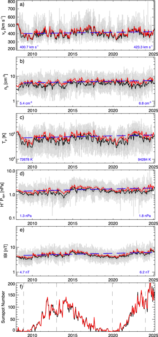
Various solar wind parameters measured at Earth’s orbital distance from 2008 to 2025. [Jasinski and Velli 2025]

Jamie Jasinski (NASA’s Jet Propulsion Laboratory) and Marco Velli (NASA’s Jet Propulsion Laboratory and the University of California, Los Angeles) analyzed solar wind data from 2008 to 2025 and found that many solar wind parameters such as speed, density, temperature, and magnetic field strength increased over that time period. This increase ran counter to expectations that the Sun may be entering a historically low period of activity in 2008.

Why it’s interesting:

The Sun undergoes an 11-year activity cycle that is driven by a change in its internal magnetic field structure. As the Sun’s magnetic activity changes, the number of sunspots, the frequency of solar flares and coronal mass ejections, and the intensity of the solar wind vary as well. Atop these mostly regular 11-year changes are longer-term variations. A recent example of this longer-term behavior began in the 1980s, when an overall weakening trend was stamped upon the usual 11-year cycle. This decline led to an exceptionally deep solar minimum in 2008, leading researchers to suspect that the Sun’s activity level might remain low for decades.

The historical context for a prolonged weak period:

Though the Sun reversed its weakening activity trend in 2008, a prolonged period with little solar activity wouldn’t have been unprecedented. Astronomers have monitored and counted sunspots for centuries, allowing modern-day researchers to investigate the Sun’s behavior long before spacecraft began to study our home star. In the historical record, there are two instances of weak solar activity spanning multiple decades: the Maunder minimum in 1645–1715 and the Dalton minimum in 1790–1830. Compared to the 11-year solar cycle, these longer-term behaviors are more difficult to predict, and their causes are uncertain.

Citation

Jamie M. Jasinski and Marco Velli 2025 ApJL 990 L55. doi:10.3847/2041-8213/adf3a6

The post Selections from 2025: The Sun Changed Course in 2008 appeared first on AAS Nova.

Featured Image: Mother’s Day Superstorms

28 July 2025 at 17:00

closeup of a solar active region

solar active regions

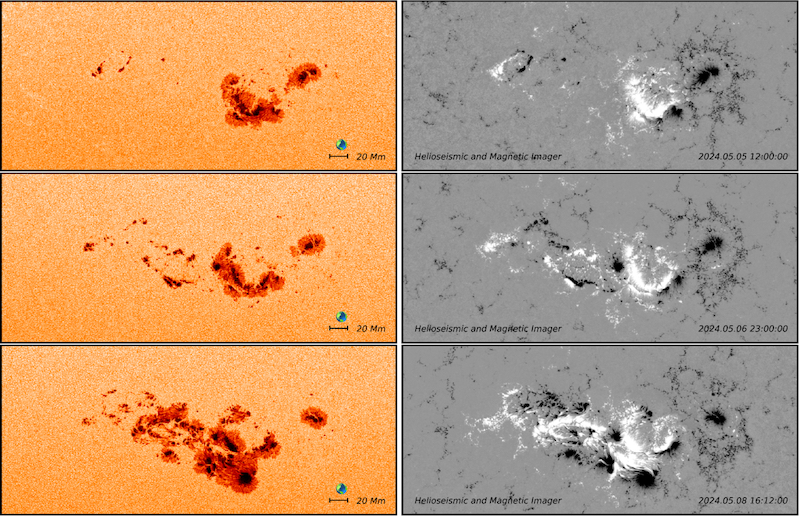
Evolution of a cluster of active regions as seen in continuum emission (left column) and radial magnetic field (right column). Click to enlarge. [Dikpati et al. 2025]

Around Mother’s Day (12 May) last year, the Sun put on a spectacular display of solar activity. A clash between solar active regions incited 14 coronal mass ejections, launched multiple high-energy X-class solar flares, and sent shimmering aurorae as far south as Florida. The images above and to the right show the source of all this excitement: the active regions AR 13664 and AR 13668. In a recent research article, Mausumi Dikpati (High Altitude Observatory) and coauthors examined the origins of this cluster of active regions and why they were such a powerful source of solar storms. Their investigation showed that there are certain regions on the Sun where solar storms are more likely to arise. These regions occur where the Sun’s undulating bands of magnetic activity draw farthest apart, preventing oppositely directed magnetic fields from canceling one another out. In the case of the Mother’s Day superstorms, active regions 13664 and 13668 developed on the heels of a decaying active region, further contributing to their magnetic complexity. Ultimately, this analysis suggested that it may be possible to forecast damaging solar activity weeks in advance by predicting the locations of magnetically complex active regions and following their evolution. To learn more about the active regions that gave rise to the Mother’s Day superstorms, be sure to check out the full article linked below.

Citation

“Mother’s Day Superstorms: Pre- and Post-Storm Evolutionary Patterns of ARs 13664/8,” Mausumi Dikpati et al 2025 ApJ 988 108. doi:10.3847/1538-4357/addd09

The post Featured Image: Mother’s Day Superstorms appeared first on AAS Nova.

❌