❌

Normal view

Astronomers Find the Strongest Evidence Yet That Alien Planets Have Magnetic Fields

8 June 2026 at 12:02
Illustration of the Sun and Earth with magnetic field lines in space.The winds on seven hellish alien worlds are moving in the wrong direction. That strange anomaly just cracked open one of exoplanet science's biggest mysteries.

When Winds Collide: Predicting the Effects of Stream Interaction Regions

14 January 2026 at 17:00

Illustration of the solar wind interacting with Earth's magnetic field

What happens when pileups of solar wind plasma collide with Earth’s protective magnetosphere? New work uses machine learning to examine how strongly these events affect our planet’s magnetic field.

Plasma Pileups

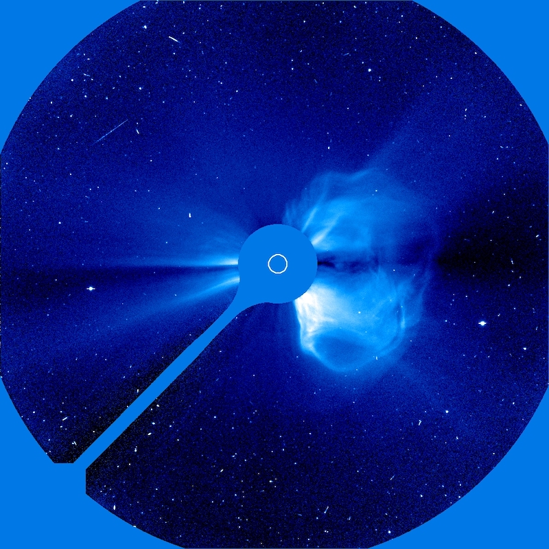
photograph of a coronal mass ejection

The Solar & Heliospheric Observatory (SOHO) took this coronagraphic image of a coronal mass ejection on 20 April 1998. [SOHO (ESA & NASA)]

Geomagnetic storms driven by solar activity paint night skies with glowing aurorae, but they also threaten spacecraft electronics with showers of high-energy particles. While immense eruptions of solar plasma and magnetic fields called coronal mass ejections are the most infamous example of solar activity, a team led by Yudong Ye (Sun Yat-Sen University) recently focused on another, less destructive form of activity: stream interaction regions.

Stream interaction regions arise when slow-moving solar wind is struck from behind by faster-moving solar wind emitted later. The collision of the two solar wind streams creates a tangle of compressed plasma and strong magnetic fields capable of peeling back Earth’s protective magnetosphere and dumping in high-energy charged particles, with beautiful yet harmful results.

Machine Learning Method

Though stream interaction regions are less disruptive than coronal mass ejections, they’re far more common; they frequently needle Earth’s magnetosphere, especially during the calmer years of the Sun’s activity cycle. Predicting how strongly a stream interaction region will influence Earth’s magnetosphere — in other words, how geoeffective it is — is challenging, however. When two streams of solar wind collide, their properties combine in complex and nonlinear ways that traditional statistical investigations have struggled to pin down.

Now, Ye and collaborators have used machine learning to study the properties and impact of stream interaction regions in a physically meaningful way. They performed their study on a sample of 879 stream interaction events for which there is abundant information, such as temperature, magnetic field strength and direction, and solar wind conditions before and after the event.

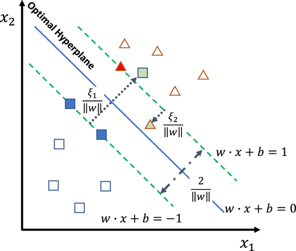
illustration of the support vector machine framework

Illustration of the authors’ support vector machine framework. The optimal hyperplane is the boundary that best divides the data by maximizing the distance between the boundary and the data points nearest to it; these points are called support vectors. Square and triangle symbols represent two classes of data. Click to enlarge. [Ye et al. 2025]

Ye’s team based their framework on a support vector machine classifier: a classical machine learning algorithm that draws a mathematical boundary between groups of data while maximizing the distance between the boundary and the data points nearest to the dividing line. The support vector machine algorithm is well-suited to the task of modeling the geoeffectiveness of stream interaction regions because it doesn’t require a particularly vast dataset, can tolerate misclassified events, and allows for a physical interpretation of the results.

A Physical Interpretation

The team first reined in the model’s complexity by identifying the most important features in the dataset. They then determined which features or combination of features had the largest contribution to the output — in other words, which physical parameters most strongly determined the geoeffectiveness of the event.

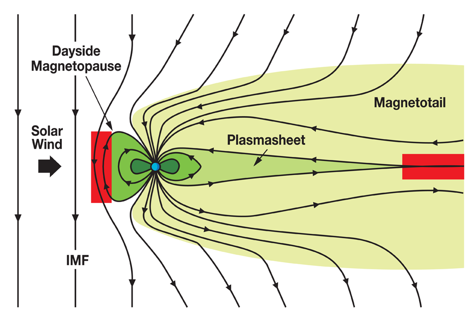
illustration of magnetic reconnection in Earth's magnetosphere

Illustration of how the interplanetary magnetic field (IMF) interacts with Earth’s magnetosphere. When the IMF points southward, as it does in this diagram, the impact on Earth’s magnetosphere is increased, with magnetic reconnection occurring in the red areas. Click to enlarge. [NASA]

Ye and collaborators found that the strongest determinants of an event’s geoeffectiveness were how long the solar wind was directed southward, the strength of the solar wind electric field, and the average and minimum strengths of the southward-pointing solar wind magnetic field. These results align with the current understanding of how energy is transferred from the solar wind to Earth’s magnetosphere through magnetic reconnection, a release of magnetic energy driven by rearrangement of magnetic fields. This shows how classical machine learning methods can enhance our ability to predict the outcome of oncoming space weather while simultaneously examining the physical drivers of the event.

Citation

“Assessing the Geoeffectiveness of Stream Interaction Regions Through Physically Interpretable Machine Learning,” Yudong Ye et al 2025 ApJ 993 10. doi:10.3847/1538-4357/ae0454

The post When Winds Collide: Predicting the Effects of Stream Interaction Regions appeared first on AAS Nova.

Minding the Gaps in Solar Wind Data

9 July 2025 at 17:00

solar wind

Spacecraft scattered throughout the solar system keep tabs on the solar wind, but the measurements are dotted with data gaps. How can scientists prevent these gaps from biasing their studies of the solar wind?

Sampling the Solar Wind

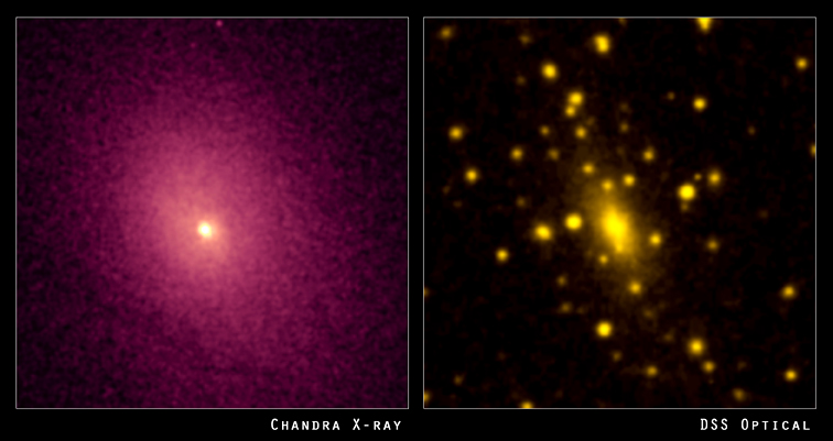
intracluster medium

Left: the distribution of hot gas between the galaxies in the cluster Abell 2029. Right: the visible light from the galaxies in the cluster. [X-ray: NASA/CXC/UCI/A.Lewis et al. Optical: Pal.Obs. DSS]

The solar wind is a tenuous, fast-moving, turbulent plasma that constantly streams out from the Sun. Studying the solar wind is important for understanding how potentially damaging space weather events like coronal mass ejections travel through the solar system. Solar wind studies also have far-reaching implications, since solar-wind-like plasmas exist throughout the universe, such as in the sparse medium between galaxies in a cluster.

Luckily, there are many spacecraft that sample the solar wind from various locations within our solar system. Unluckily, many of these spacecraft do not continuously monitor the solar wind. For example, when a spacecraft orbiting a planet dips into the planet’s atmosphere, this detour creates an hours-long gap in solar wind monitoring.

The Impact of Data Gaps

How do these data gaps affect studies of the solar wind? In a recent research article, Daniel Wrench and Tulasi Parashar (Victoria University of Wellington) approached this question in terms of how gaps affect the structure function: a mathematical description of how the solar wind fluctuates over different length or time scales.

Wrench and Parashar introduced random artificial gaps into data from the Parker Solar Probe, which monitors the solar wind continuously, and compared the structure functions calculated from the continuous and interrupted data sets. They used the difference between the true structure function — calculated from the continuous data set — and the structure functions from the artificially gapped data sets to develop a correction factor.

bar plot of correction method performance

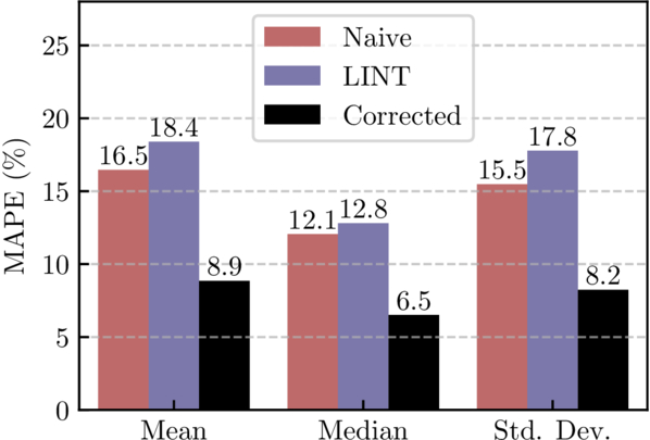
Performance of the correction factor method (black) compared to the uncorrected, gapped data (red) or gaps filled using linear interpolation (blue). MAPE is the mean absolute percentage error. [Wrench & Parashar 2025]

The team then tested their correction factor using data from the Wind spacecraft, which continuously monitors the solar wind from the L1 Lagrange point. The team calculated the structure function from 1) the continuous data set, 2) the artificially gapped data, 3) the gapped data with linear interpolation used to fill the gaps, and 4) the gapped data with the correction factor applied. This test showed that the correction factor performs better than other commonly used gap-handling methods, such as linear interpolation, which can systematically underestimate the structure function. Using the correction factor, the error in the structure function remained below 50% even when 95% of the data were missing.
plot of structure function from Voyager 1 data

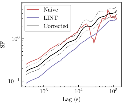
Structure function calculated from uncorrected Voyager 1 data (red), linearly interpolated data (blue), and corrected data (black). Both the linear interpolation method and the correction factor method remove the artifact around a lag of 3×10⁴ seconds, but the correction factor method does not suppress the signal like the linear interpolation method does. [Adapted from Wrench & Parashar 2025]

Correcting Voyager 1

Finally, the authors applied their validated method to data from Voyager 1. Data from the two Voyager spacecraft are extremely scientifically valuable — no other spacecraft have ventured as far from the Sun and can measure the solar wind at such large distances. The data are also extremely sparse; one segment used in this work was missing 85% of the data. This means that an effective method of correcting these data has potentially huge scientific significance.

Wrench and Parashar applied their correction factor to the Voyager 1 data, showing that this method handily removes artifacts while avoiding the underestimation introduced by linear interpolation. While the authors saved the interpretation of the newly corrected Voyager 1 data for future research, this study makes it clear that even large data gaps needn’t hinder studies of the solar wind.

Citation

“Debiasing Structure Function Estimates from Sparse Time Series of the Solar Wind: A Data-Driven Approach,” Daniel Wrench and Tulasi N. Parashar 2025 ApJ 987 28. doi:10.3847/1538-4357/addc6a

The post Minding the Gaps in Solar Wind Data appeared first on AAS Nova.

❌