 Login

Researchers develop plant-based scaffold to grow cultivated meat in lab
A team of researchers at McMaster University have produced a new plant-based, edible scaffold for cultivated meat that

Billions of people still suffer from hunger and food insecurity worldwide. Meanwhile, microbial contamination causes a third of global food waste annually, resulting in major economic losses and illnesses. Although antibiotics and pesticides help control contamination, their excessive use can promote bacterial resistance or leave toxic residues.
One alternative uses materials that generate highly reactive forms of oxygen when exposed to light, called photocatalysts, to prolong food freshness. These molecules kill bacteria by damaging their cell components in a process called photodynamic inactivation or PDI. However, current PDI systems rely on energy-intensive lasers and long exposure times because the bacteria’s protective cell membranes block reactive oxygen molecules. As a result, the systems don’t kill bacteria effectively and risk overheating food, affecting its freshness and nutritional value.
Scientists at Zhejiang University in China thought that it would be possible to achieve a PDI system using accessible, free sunlight with the right photocatalyst. Moreover, they also wanted to integrate this photocatalyst into food packaging to combat microbes during storage.
To make the photocatalyst, the researchers mixed water with a glue-like plant fiber that provides structural support, called pectin, and a chemical from plant seeds that supplies phosphorus, called phytic acid. Then they heated the mixture in a sealed reactor at 220ºC (428ºF) for 5 hours to form tiny structures composed of a carbon core surrounded by a phosphorus-rich shell called phosphorus-modified carbonized polymer dots or PCDs.
To incorporate the PCDs into film packaging, the researchers dissolved equal amounts of a plant fiber from konjac, called glucomannan, and another plant-derived molecule, called carboxymethylcellulose, in warm water to form a network of entangled molecular chains. Then, they added 1.5 milligrams of PCD per milliliter to this mixture, which linked the chains together like molecular fasteners. Finally, they added a moisture-binding chemical called glycerin to prevent brittleness. The researchers cast this mixture onto separate Petri dishes and dried them, forming thin, plastic-like PCD films.
To test the films, the researchers placed Escherichia coli bacteria between 2 sterilized film sheets and exposed the samples to either darkness or simulated sunlight for 20 minutes. They then transferred the microbes onto agar plates and incubated them for 15 hours, allowing surviving bacteria to form visible colonies. They compared the number of bacterial colonies with those of untreated samples to calculate the percentage of bacteria the films eliminated in each environment.
Tests under darkness showed that the films eliminated about 60% of the bacteria. The researchers attributed this result to the positive electrical charge of PCDs, which attracts the bacteria’s negatively charged cell surfaces. The electrical attraction stresses their cell membranes, interfering with essential life processes. This result suggested that the films use a separate charge-based antibacterial mechanism apart from PDI, which requires light to work.
Under simulated sunlight, the films eliminated nearly 100% of the bacteria. The researchers identified 2 principal mechanisms causing this. First, the PCDs acted as tiny heaters that generated localized heat, which stretched holes in the bacterial membranes, allowing contents to leak out of their cells through a process called photoporation. Second, the PCDs generated reactive oxygen molecules that could then penetrate the bacteria. Once inside the cells, these molecules irreversibly damage the bacteria’s internal components and genetic material through PDI.
The researchers also investigated whether PCD films could serve as food packaging by using them to wrap fresh strawberries. Compared with conventional nonbiodegradable polyethylene packaging where visible rotting occurred, the PCD films kept the strawberries fresh for more than 4 days by suppressing bacterial growth and regulating moisture levels. When the team tested whether the films were toxic, they found that the films are safe for humans and compatible for food applications. They also buried the films in soil for 24 days and found that they degraded by 78%, demonstrating biodegradability suitable for packaging fresh foods.
The team concluded that PCD films could be a biodegradable food packaging that combines plant-based materials with multiple antibacterial strategies. The films retained antibacterial activity in darkness and became more effective under sunlight through the combined effects of photoporation and PDI. These findings demonstrated that by combining multiple mechanisms into a single material, researchers can create multifunctional food packaging that remains effective across different storage conditions.
The post Harnessing sunlight to fight bacteria appeared first on Sciworthy.
Drilling for electricity or geothermal energy is a common human-caused source of earthquakes. Drillers or engineers inject water into the earth to fracture underground rock through a process known as fracking. This allows scientists to produce clean energy almost anywhere on Earth by heating up water in the cracks using facilities called enhanced geothermal systems or EGS plants. However, fracking causes earthquakes, which are a major concern for people’s safety globally. Therefore, scientists are looking for new fracking methods that cause fewer earthquakes.
Fracking for EGS plants can trigger earthquakes by changing the pressure underground and adding stress to the surrounding rock. However, these earthquakes happen at pre-existing, naturally occurring cracks called faults, which are different from the newly formed, man-made cracks. Faults are naturally under pressure from the overlying rock and the surrounding earth since they reach deep underground. As pressure builds up over time, it eventually causes the rocks to shift along these faults and release energy in the form of earthquakes.
During fracking, engineers use 4 different shut-in strategies to finish off water pumping. The standard industry strategy is called instant shut-in, where the injection pump is turned off immediately, but the water stays underground, causing the pressure to lower naturally. In a similar strategy, known as the tapered shut-in, engineers gradually reduce the water injection rate to zero instead of immediately turning it off. For the high-rate and low-rate extraction strategies, they pump the water back out after injection is complete, at different pump rates.
Recently, scientists aimed to mitigate the risk of earthquakes by testing these 4 shut-in strategies to determine which is most effective. They compared the shut-in strategies using crystalline basement rock with low porosity and permeability, meaning water couldn’t easily flow through it. Engineers use this same type of rock for EGS plants so they can control where the water flows. The scientists pumped water into the rock, then measured the pressure and stress levels where rocks began to move along faults, determining the point at which earthquakes would occur.
The scientists applied high-rate and low-rate extraction methods to the rock and found that pressure and fault movements decreased. However, when they applied instant and tapered shut-in methods to the same rock, they increased the pressure and caused continuous fault slipping. They measured stress in the rock during these methods and found that high-rate extraction stabilized the fastest, while low-rate extraction stabilized more slowly. In contrast, instant shut-in continuously increased the pressure and slip, and tapered shut-in caused the highest stress of all.
The scientists also used a computer model to simulate what happened at an EGS site in South Korea, where earthquakes occurred after injections using the instant shut-in method. They set up the model using a rock with the same characteristics, injection wells, and faults as that site. Then, they simulated periods of injection based on the previous real-world events and modeled the effects of pressure and stress to determine if the earthquakes could have been prevented.
The team used the model to compare how a site like this would respond to the instant shut-in method versus the other shut-in methods. They found that the tapered shut-in method increased pressure and stress in the rock, while the high-rate and low-rate methods both decreased pressure and stress. The high-rate method decreased pressure and stress more than the low-rate method.
The scientists concluded that high-rate extraction is the most effective method for reducing the risks of post-injection earthquakes during EGS fracking in crystalline basement rock. Additionally, the scientists determined that the earthquakes in South Korea could have been prevented if engineers had used either the high-rate or low-rate extraction methods. They recommend using high-rate extraction to reduce earthquakes during EGS fracking, which would allow EGS plants to generate clean energy more safely.
The post Reducing earthquakes caused by fracking appeared first on Sciworthy.
Beyond the solar system, the line between planet and star can get blurry. Astronomers call objects that fall between the size ranges of planets and stars substellar objects. One type of substellar object, called a brown dwarf, forms from collapsing gas clouds like a star, but is not quite massive enough to fuse hydrogen in its core. Some can briefly fuse a heavier form of hydrogen, known as deuterium, in their cores, though never enough to produce starlight. Others are small and cold enough to develop complex atmospheres.
Recently, astronomers discovered a new type of substellar object in a star-forming region of the Milky Way Galaxy called IC 348. Using observational data from the JWST’s Near InfraRed Spectrograph (JWST NIRSpec), they found objects 0.2% to 1.2% the mass of the Sun that float freely like stars but have carbon-containing molecules called hydrocarbons in their atmospheres. Because these objects are smaller than known brown dwarfs and have evidence of hydrocarbons, scientists refer to them as H-type objects.
To investigate what H-type objects are and where they fit within the spectrum of substellar objects, researchers Richard J. Parker and Catarina Alves de Oliveira analyzed survey data on stars and substellar objects in IC 348, then conducted follow-up simulations to uncover how H-type objects formed. The main question they asked was whether H-type objects form from collapsing gas clouds, like brown dwarfs and stars, or develop around host stars before being ejected and drifting freely through space, like planets.
First, they reviewed the observational records of IC 348 obtained with the JWST NIRSpec and the near-IR spectrograph SpeX at the NASA Infrared Telescope Facility. IC 348 has 495 stars and brown dwarfs combined, as well as 9 H-type objects. Estimates for the age of this star-forming region range from either 1 to 3 million years or 5 to 6 million years, depending on how different teams calculated it. From there, Parker and Alves de Oliveira compared where the stars, brown dwarfs, and H-type objects were located within the cluster. They found no unique spatial distribution among the 3 types of objects.
Then, the team simulated the evolution of IC 348 over 10 million years to determine which initial conditions would result in a spatial distribution closest to the survey data. They simulated an initial giant gas cloud and used a mathematical function to distribute its mass among the 495 constituent objects. The researchers then placed a Jupiter-sized planet around each simulated star that was approximately the Sun’s mass to determine whether they could grow and escape their home star and become H-type objects. They also repeated the simulations by placing the Jupiter-sized planets at distances from the Sun similar to those of Earth, Jupiter, and Neptune, and varied the sizes and star densities of the simulated IC 348 regions.
They found that if Jupiter-sized planets orbited their stars at roughly Jupiter’s distance from the Sun, then 5 to 15 of them could escape their stars in a region like IC 348, which would roughly match the number of known H-type objects. However, the escaped planets were distinctly more spread-out than the observed H-type objects, which share a similar spatial distribution with the cluster’s stars and brown dwarfs. Since the simulations did not match the observed distribution, the researchers suggested that these H-type objects are likely a new sub-category of very small brown dwarfs rather than escaped planets.
Although this study favors a brown dwarf origin for H-type objects, the exact details of how they formed remain up for debate. Astronomers still have multiple competing theories about how ordinary brown dwarfs form. Perhaps they are ejected from their gas cloud before fully forming, have their outer layers stripped by radiation from a nearby massive star, or simply form like stars on a slightly smaller scale. Regardless, future researchers will continue to explore this murky area of substellar astronomy.
The post Objects at the border between planets and stars appeared first on Sciworthy.
Since the formation of the Earth 4.2 billion years ago, hot rock from the interior of the planet has cooled off and developed crystals that accumulated over millions of years, forming surface rocks with a layered composition, referred to as continental crust. Geologic evidence of how continental crust formed comes from large, ancient crustal blocks, called cratons. Cratons have existed for billions of years and form the cores of continents.
Scientists have shown that the upper 10 to 15 kilometers (6 to 9 miles) of continental crust contains high concentrations of elements like uranium and thorium that decay and release heat over time, referred to as radiogenic elements. However, the lower 20 kilometers (12 miles) of crust has very few radiogenic elements. The cause of this planetary-scale differentiation is highly questioned, as geoscientists don’t know what formation processes could produce this unique characteristic.
Earlier researchers suggested that changes in the concentration of radiogenic elements could occur when tectonic plates collide. Plate collision induces temperatures in the lower crust high enough to melt minerals that contain uranium and thorium, like zircon and monazite. The newly melted minerals form magma, which then rises and crystallizes in the upper crust. To test whether this process formed the layered continental crust, researchers Andrew J. Smye and Peter B. Keleman incorporated geochemical data from studies worldwide into a mathematical model comparing how concentrations of radiogenic elements vary under different temperatures.
The team separated their global analyses into 2 categories of rocks that were buried deep in the crust and subjected to intense pressures and temperatures, via a process known as metamorphism. The first category included rocks formed from the accumulation of eroded grains buried in the deep crust that are subjected to high pressures and temperatures, called metasedimentary rocks. The second category included rocks formed when magma rises from the deep Earth and solidifies before experiencing high pressures and temperatures, called metaigneous rocks.
The researchers analyzed 3 subcategories from each of the 2 types of deep-crustal rocks. The first was rocks that experienced no intense pressure or temperature, the second was rocks subjected to 650 to 900°C (about 1,200 to 1,650°F), and the third was rocks subjected to 900 to 1,100°C (about 1,650 to 2,000°F). The researchers modeled the geochemistry of the 3 rock types at different temperatures to determine whether ultra-high-temperature metamorphism could cause crustal differentiation of radiogenic elements.
Smye and Keleman found that monazite doesn’t melt in either metasedimentary or metaigneous rocks at temperatures below 900°C, as indicated by the relatively high thorium content in these deep-crustal rocks. Alternatively, they found that above 900°C, uranium and thorium concentrations decreased in metasedimentary rocks, suggesting that minerals like zircon and monazite were melting. The melted minerals enter magma and rise into the upper crust, leaving behind metasedimentary rocks depleted in radiogenic elements by around 0.10 ppm.
The team concluded that the enrichment of uranium and thorium in the upper continental crust requires temperatures greater than 900°C to initiate the melting of zircon and monazite in the lower crust. Temperatures above 900°C are linked to the movement and collision of continental plates. This result suggests that evidence of Earth’s differentiation has been preserved for more than 3 billion years, spanning most of the planet’s geological history. Since stable continental crust formed, uranium and thorium enrichment in the upper crust has consistently recorded layering produced by ultra-high temperature metamorphism.
The post Why is Earth’s crust layered? appeared first on Sciworthy.
Diseases that cause nerve cells in the brain to die over time are known as neurodegenerative diseases. These cells, known as neurons, are vulnerable to DNA damage because they are highly active cells that require large amounts of energy. Neural DNA damage is a normal part of aging as changes to the DNA sequence, called mutations, build up over time.
Previous scientists have shown that neurons from people with the neurodegenerative diseases Alzheimer’s disease (AD), frontotemporal dementia (FTD), and amyotrophic lateral sclerosis (ALS) accumulate unusually high numbers of changes in the DNA sequence, called somatic mutations. However, researchers don’t know what causes the high number of mutations or whether the same process causes them in all 3 diseases.
To answer these questions, researchers at Boston Children’s Hospital and Harvard Medical School analyzed brain tissue from people who died with and without AD, FTD, or ALS. They compared the processes that cause DNA mutations in the 3 diseases by first accessing the DNA inside individual neurons from healthy and diseased postmortem brain tissue.
To do this, they broke apart the brain tissue and added a fluorescent marker that identified the center of each neuronal cell where DNA is housed, called its nucleus. They used a sorting machine to separate the nuclei from the rest of the cell material to access the neuron’s DNA. Using a DNA sequencing method called single-cell whole genome sequencing, the team then sequenced each neuron’s DNA to identify mutations.
They analyzed 159 neurons from people with AD, 61 neurons from people with FTD, 77 neurons from people with ALS, and 232 neurons from healthy individuals. This allowed the team to compare the number and types of DNA mutations between diseased and control (non-diseased) neurons. The researchers found that compared to the control neurons, which typically accumulate only 200 to 300 mutations over an 80-year lifespan, neurons from all 3 diseases contained an unusually high number of 2-base-pair deletions, often exceeding 1,000 mutations per cell.
When a biological process damages DNA, it leaves behind its own unique signature. By identifying these signatures, scientists can identify the biological process that likely caused the damage. Since these 2-base-pair deletions were so frequent in diseased neurons, the researchers wanted to know whether they were left behind by a biological process. The researchers used a machine learning algorithm to scan DNA sequences for recurring mutation patterns and identified a signature in neuronal DNA, which they named ID-4.
When the researchers compared the ID-4 signature with a database of previously characterized signatures, they found that it was associated with a DNA repair protein called TOP1. TOP1 temporarily cuts and rejoins DNA to relieve the tension that builds up during normal cellular activity. TOP1 typically detaches from the DNA after completing this process. However, if TOP1 fails to detach, it breaks one of the two DNA strands.
To test whether abnormal TOP1 activity was breaking the DNA, the researchers isolated DNA from control and diseased neurons. They visualized the DNA on a gel, where intact DNA forms bands while broken DNA spreads out into smears. The more fragmented the DNA is, the more intense the smear appears. Using a machine that quantified the intensity of smears, the researchers found that DNA from diseased neurons produced smears that were up to 3.2 times more intense than those from control neurons. They also found that neurons with more DNA fragmentation had more ID-4 signatures.
Based on these findings, the researchers concluded that abnormal TOP1 activity created frequent single-strand DNA breaks. They proposed that some of these breaks are repaired incorrectly, eventually leading to widespread DNA breaks in all 3 neurodegenerative diseases.
Overall, the researchers found that neurons from these 3 neurodegenerative diseases accumulated excessive DNA mutations despite differences in the disease symptoms and underlying causes. Their findings also provided evidence that abnormal TOP1 activity contributes to this mutation accumulation. Based on these findings, they stated that preventing TOP1 from becoming trapped on DNA, or improving the DNA repair process that removes trapped TOP1, could be a promising way to treat a wide range of neurodegenerative diseases.
The post Common DNA damage could cause neurodegenerative diseases appeared first on Sciworthy.
Since the 1850s, plowing and clear-cutting in modern agriculture have increased how fast soil erodes in the Upper Mississippi River Valley. Across the globe, farming strips soil up to 100 times faster than natural processes. It also removes farmable land and clogs waterways, threatening long-term environmental sustainability. However, scientists in the past have struggled to separate the effects of land-use changes from the transition out of the last ice age over the past 20,000 years.
To determine whether current farming practices are sustainable, researchers from Minnesota recently measured the speed at which soil eroded during the ice age transition and compared it with modern agricultural erosion. They focused on the Trout Creek tributary of the Mississippi River. This tributary has 2 step-like formations, or terraces, on its bank that represent past floodplains before the river eroded to its current level.
The oldest, upper terrace is about 14 meters (50 feet) above the lower terrace, which is about 8 meters (26 feet) above the modern floodplain. Scientists studying nearby areas have suggested that the terraces contain sediment from the last ice age, 20,000 years ago, referred to as the Last Glacial Maximum, to today.
In the upper terrace, the researchers pushed an empty cylinder into the ground, like a straw into a layer cake, to collect a cylindrical sample of sediments about 4 centimeters (1.5 inches) wide and 6 meters (20 feet) deep, called a sediment core. They collected slices of this core from 2 meters (6 feet) and 6 meters (20 feet) to find the terrace’s age.
Some grains in the sediment trap electrons while buried and release them when exposed to light. So the team shone light on the sediment slices to stimulate these electrons and measure the intensity of light emitted, known as their optically stimulated luminescence. Brighter light emissions indicate the sediment is older and was buried for a longer period of time. Using this method, they confirmed that the deep sediment slice was 22,000 years old, and the shallow sediment slice was 20,000 years old, dating the terrace back to the Last Glacial Maximum.
Next, the team drilled into the upper terrace with an auger to collect 25-centimeter (10-inch) wide plastic tubes of sediment. They pulled 4 samples from 0 to 2 meters (0 to 6 feet), and 1 sample from 6 meters (20 feet) deep. They explained that minerals in the sediment called quartz produce the radioactive form of the element beryllium, known as 10Be, when exposed to the Sun, so low 10Be means the sediment was buried quickly and had little sun exposure. The team measured the concentration of 10Be in each sediment sample and used an online calculator to estimate how quickly it eroded. The researchers calculated that during the Last Glacial Maximum, 0.073 millimeters (0.003 inches) of surface sediment were removed per year.
The researchers collected similar samples from the lower terrace and used optically stimulated luminescence to determine that it was between 22,000 and 14,000 years old. This terrace was the floodplain during the transition out of the Last Glacial Maximum, or deglacial period, where temperatures warmed and permafrost retreated. They measured the concentration of 10Be in samples from this terrace and determined that 0.049 millimeters (0.002 inches) of surface sediment were removed per year.
Finally, the researchers measured 10Be in a sediment sample from the modern floodplain, deposited between 14,00 years ago and today. They found that the sediment had eroded 0.053 millimeters (0.002 inches) per year during that interval, at a rate slower than it had during the glacial period, but similar to the deglacial period.
The researchers compared their findings to the average soil loss caused by modern agriculture, as reported by 4 previous scientists studying the area. They saw that modern farming removes an average of 0.60 millimeters (0.02 inches) of soil per year, which is 8 to 12 times greater than all the natural erosion rates they calculated.
They concluded that the recent spike in soil loss from agriculture greatly exceeds that caused by the largest natural climate transition in recent Earth history. Human-driven erosion shows an upward “hockey stick” trend like the one seen in global temperatures, suggesting that similar trends could exist throughout Earth systems. The team concluded that modern agricultural practices aren’t currently sustainable. While measures like native plant reintroduction can help curb this trend, more research is required to determine how best to limit long-term erosion.
The post Is modern farming sustainable? appeared first on Sciworthy.
In the 1970s, astronomer Vera Rubin analyzed a series of observations of how quickly different galaxies rotated around their centers. She found that these galaxies rotated much faster than they should have, given the amount of material visible through starlight. She concluded that a large fraction of these galaxies’ masses must therefore consist of some kind of unseen material.
Scientists have since observed galaxies to more precisely measure this unseen material, which they now call dark matter. They’ve shown that dark matter moves much more slowly than the speed of light. Unlike most celestial objects, it can’t emit or block any light, meaning it doesn’t interact with the electromagnetic force. Even though it doesn’t interact with a fundamental force in the universe, dark matter constitutes over 80% of the mass of an average galaxy.
In the prevailing model of cosmology, known as ΛCDM (pronounced “Lambda-CDM”), dark matter determined where galaxies formed. The theory is that gravity pulled dark matter together more quickly than regular matter in the primordial universe. This redistribution led to regions of space with greater mass density, which collected chaotic, regular matter into pools that eventually formed galaxies, stars, and planets.
In the present universe, dark matter and regular matter coexist in galaxies, though generally separated. Regular matter pools in the very center of galaxies, forming the more familiar galactic disks. Dark matter stays towards the edges of galaxies, enveloping the regular matter disks in what are known as dark matter halos. Because these halos make up so much of the mass of the average galaxy, researchers Guangze Sun, Fangzhou Jiang, and Jing Wang conducted a series of simulations to test how dark matter halos affect regular matter in galaxies. Specifically, they examined what characteristics of dark matter halos determine galaxy sizes.
The force of gravity works such that more massive dark matter halos draw in more regular matter and produce larger galaxies. So these researchers fixed the total mass of the galaxies they simulated at 100 billion times that of the Sun to determine which properties of the dark matter halos would produce the widest galaxies. They selected 4 variables to test: the total density of dark matter in the galactic halo, the density of dark matter in the innermost 1% of the halo, how fast the halo spun, and the ratio of regular matter to dark matter in the entire galaxy. For each variable, they tested 3 to 4 inputs representing low, moderate, and high values against a standard reference value and ran 132 total simulations to generate enough data for statistical analyses.
To simulate the complex physics of dark matter halos, the team used the modeling software GIZMO to model gravity, magnetism, and fluid dynamics. They combined this with a second model, called FIRE-3, which modeled how stars explode at the end of their lives, how much metal these explosions produce, and how gases heat up and cool down over time. The researchers ran the dynamic simulations for 3 billion model years, then used a program they developed based on the existing Pynbody to measure the radii of the simulated galaxies.
The team found that the faster a dark matter halo spun around a simulated galaxy, the larger the galaxy became, as shown in scenario 1 in the figure below. By contrast, in scenario 2, increasing the halo’s total dark matter concentration caused the central galaxy to shrink. Increasing only the innermost dark matter density in the halo had a smaller effect but generally reduced the galaxy’s size, as shown in scenario 3. And lastly, increasing the ratio of regular matter to dark matter in galaxies resulted in smaller galaxies that formed stars closer to their centers, as shown by a greater concentration of stars in scenario 4.
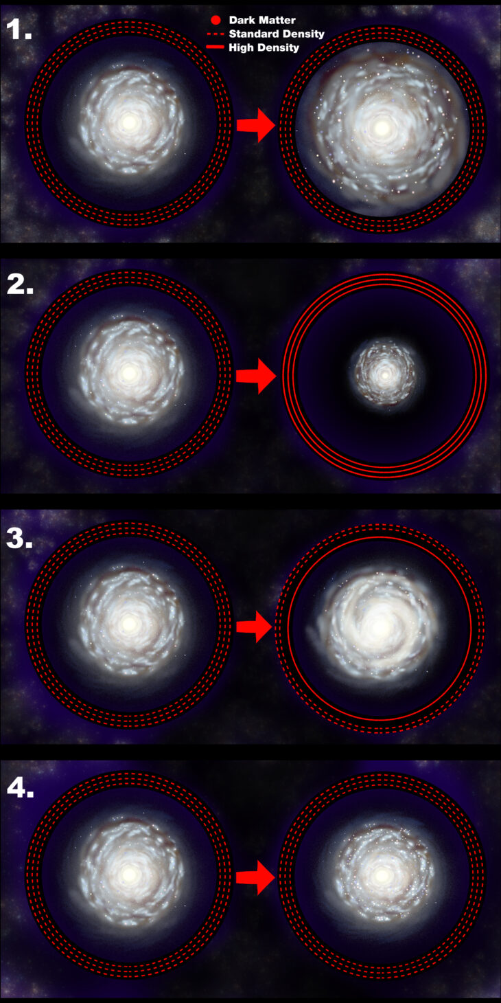
This diagram showcases the team’s results across 4 broad scenarios. The left column depicts a default galaxy under the baseline parameters. The right column depicts how the galaxies changed when the team varied a single experimental factor, including 1) increasing how fast the dark matter halo spun, 2) increasing the total density of the dark matter halo, 3) increasing the density of dark matter in the innermost halo, and 4) increasing the ratio of regular matter to dark matter in the entire galaxy. The dark matter haloes are represented as red rings surrounding the galaxies, not to scale. Illustration by Andrew Bizal.
The team’s results suggest a previously unknown connection between the properties of dark matter halos and galactic disks. However, they cautioned that their simulations were all run on galaxies in isolation, unlike in the actual ΛCDM universe, where their interactions are complicated by galaxies tugging on one another or by material moving from one to another. To further test their results for single galaxies, the researchers plan to run follow-up experiments with halos of different sizes, as well as with galaxies with different shapes and features, such as clumps, gaps, and lopsidedness.
The post Dark matter influences the size of galaxies appeared first on Sciworthy.
Temperatures in the Arctic are increasing at a rate 4 times faster than the average global temperature. Scientists have documented the global effects of climate change, but there are still regions where these effects are less well known. This is the case for freshwater ecosystems in the Arctic.
When the ground has been permanently frozen for 2 years, scientists call it permafrost. Permafrost contains soil, sand, rocks, and organic matter held together by ice. As temperatures rise, permafrost thaws, which can change groundwater flow paths. It can also alter a stream’s temperature, flow patterns, and nutrient loads by introducing new material from the permafrost.
To determine how thawing permafrost affects Arctic ecosystems, scientists from the U.S. Geological Survey recently studied 10 headwater streams within the Brooks Range in the Noatak National Preserve of Alaska. The scientists studied streams with different amounts of permafrost and ice to test whether connections exist between permafrost, food webs, and populations of fish called the Dolly Varden and Arctic Graylings. They focused on these 2 species of fish because their migrations often indicate ecological shifts in the area.
The scientists collected fish from the streams by temporarily stunning them, using a method called electrofishing, or by catching them in minnow traps. They manually identified each species they collected, then froze the fish and shipped them to a lab. Once in the lab, the scientists measured the length of each fish and used documented growth patterns to estimate its biomass. To calculate fish abundances, they divided their total biomass by the time spent electrofishing or trapping. Finally, they measured the energy density of each fish by burning it in a device called a bomb calorimeter.
At each stream, the scientists took manual temperature measurements and deployed loggers that recorded the temperature every 15 minutes. They also deployed equipment at the bottom of each stream to record water pressure in 15-minute intervals and converted the data to depth, since pressure increases with depth. Then, they used wading rods to measure how much water was flowing through each stream at a given spot.
They combined the depth and wading rod data to determine the flow rate of water in the streams over time. They used these data to identify unstable streams where water rose and fell rapidly. They also collected water samples from each stream and measured their nutrient concentrations, including dissolved organic carbon, nitrogen, and phosphorus, to determine water quality.
Finally, they measured 2 types of smaller organisms that allow energy to flow through the food web to the fish, called microbial biofilms and macroinvertebrates. They used a hand-held device to estimate the types and amounts of biofilms, and nets to collect macroinvertebrates.
Once they had compiled these data, the team conducted a statistical analysis to compare the studied parameters and fish populations to the extent of permafrost in each area. They found that streams with more permafrost in the area had warmer temperatures, because the permafrost prevented water from infiltrating the soil to cool off. The streams with warmer temperatures, in turn, had lower abundances and biomass of Dolly Varden fish and Arctic Grayling with lower energy densities. They suggested that these results meant that the high temperatures had pushed the fish above their optimum temperature range.
They also learned that the limited infiltration in permafrost areas caused rainfall to flow straight into the stream. This process created instability as the stream levels rose and fell rapidly. Fish in these unstable streams had lower energy densities, likely due to the harsher environment.
Areas with greater permafrost also had higher concentrations of dissolved organic carbon and phosphorus, which stimulated the formation of biofilms at the bottom of the food chain. They noted that areas with more biofilms also had more macroinvertebrates and more Dolly Varden biomass. Since the Dolly Varden eats macroinvertebrates, this finding suggested that the lowest levels of the food web shape the health of species higher up. This is called the bottom-up effect, and means that areas with more biofilms and macroinvertebrates will likely have healthier and larger fish populations.
The scientists explained that knowing how these factors influence Arctic fish populations can help researchers understand how thawing permafrost might affect Arctic ecosystems in the future. They anticipated that their data could help future researchers predict how these and other ecosystems will be impacted by changing landscape dynamics caused by global warming.
The post Thawing permafrost is affecting fish health appeared first on Sciworthy.
Have you ever experienced a severe weather event, like a hurricane or a tornado? Researchers have shown that climate change is causing such weather events to become more extreme and more frequent, destroying communities and infrastructure. To determine which areas are most at risk, researchers from Canada studied the environmental effects of a powerful flooding event that occurred in southwestern British Columbia (BC) in November 2021.
They focused on a type of severe flooding event that is characteristic of the North American Pacific coastal region, called an atmospheric river. An atmospheric river occurs when a long, narrow vapor cloud flows toward land from the Pacific Ocean, causing heavy rainstorms. In November 2021, an atmospheric river in southwestern BC destroyed numerous regional highways, pipelines, power lines, and railways within its path. Over 18,000 people were evacuated due to flooding, and 6 people died.
The team explained that before the storm, BC experienced a severe drought and an unprecedented heatwave, followed by widespread thunderstorm activity. In 2021, lightning and human activity caused nearly 1,000 wildfires, which led to the third-worst wildfire season ever recorded in BC, partially because trees grow back slowly in forests that have been cut down or harvested. Poor vegetation recovery makes harvested forests more vulnerable to wildfires than old-growth forests. The November atmospheric river occurred shortly after this wildfire season.
To determine how the atmospheric river impacted southwestern BC, the researchers analyzed approximately 70,000 square kilometers (27,027 square miles) of affected area. They compared satellite images of southwestern BC from Google Earth, Sentinel, and Landsat taken before and after the event to detect changes in river channels and identify geohazards, like landslides and debris flows. They also used satellite images and Canadian government data to identify which forests had been harvested within the study area. The researchers then traversed the area to confirm their remote analyses.
The researchers used a type of 3D remote sensing, called light detection and ranging, or lidar, to measure how the 2021 atmospheric river redistributed sediment in the Coquihalla and Coldwater River valleys. With the help of lidar, the researchers discovered that both rivers had severely unstable banks due to erosion from the flooding event. Along the Coquihalla River, approximately 53,000 cubic meters (1,871,677 cubic feet) of sediment were eroded, while nearly 50,000 cubic meters (1,765,733 cubic feet) of sediment were eroded along the Coldwater River.
The researchers also found that hillslope geohazards increased the volume of sediment in both rivers. And in some cases, upstream areas with a history of forest harvesting and wildfires also affected stable banks downstream. For example, they identified debris flows on an unstable hillslope that triggered a landslide on a riverbank downstream. They observed that the river and stream channels shifted due to a sudden addition of sediment from hillslope geohazards and floodwater during the event.
In total, the researchers documented over 1,300 geohazards along 47 kilometers (about 30 miles) of the Coquihalla River and 19 kilometers (about 12 miles) of the Coldwater River and nearby creeks. Nearly half of the geohazards originated in an area with a history of wildfires or forest harvesting. Of the 155 geohazards at the Coquilhalla River, 43% occurred below forest harvesting resource roads, and of the 117 geohazards observed at the Coldwater River, 29% originated in areas with past wildfires.
The researchers suggested that their findings could help scientists predict where severe geohazards will occur during extreme weather events, since both watersheds had geohazards originating in harvested forests. Before 2000, clear-cutting was a widespread practice in BC, and the team’s results demonstrate that unsustainable harvesting practices like this can have lasting environmental impacts.
The researchers concluded that both forest harvesting and wildfires contributed to the severe impacts of the November 2021 atmospheric river, causing catastrophic landslides and debris flows to occur in traditionally dry regions. They suggested that more accurate risk assessments can better equip communities for severe weather events like this. While the next atmospheric river that lands in the Pacific coastal region may be worse than the last, this study can inform scientists and communities about which areas it might affect most.
The post Wildfires and forest harvesting worsen severe weather impacts appeared first on Sciworthy.
Horseshoe crabs are marine animals more closely related to spiders than crabs. These animals have existed for more than 450 million years, and are sometimes called “living fossils” because they appear to have changed very little throughout their evolutionary history. However, horseshoe crabs have a poor fossil record, so this apparent lack of change could also be due to a lack of evidence, particularly when it comes to their reproduction. Scientists want to know: Are horseshoe crabs truly living fossils?
Modern horseshoe crabs reproduce by releasing hundreds of eggs and sperm into tidal waters, via a process called external fertilization. Until now, scientists have assumed that horseshoe crabs have always reproduced this way. But paleontologists have only found 3 fossil horseshoe crabs from the past 252 million years with their reproductive systems preserved, so this assumption is mainly based on an absence of evidence to the contrary.
Scientists in the past interpreted the horseshoe crab’s long history of external fertilization as indicative of its evolutionary consistency. However, James Lamsdell and colleagues recently discovered a new fossil species of horseshoe crab in the 450 million-year-old Big Hill Formation in Michigan that challenges this assumption.
To study the specimen, the scientists photographed it under 2 types of microscopes. The first type of microscope used polarized light to see structures in the fossil that may have blended into the rock, like putting on special glasses to see subtle textures. The second type of microscope used fluorescent light to reveal soft tissue in the fossil. Only some tissues, like ovarian tissue and preserved eggs, glow under fluorescence, so this method helped the team rule out non-biological structures, like bubbles, cracks, or minerals.
The researchers found that their analytical techniques revealed remarkable details about the ancient horseshoe crab. One unique feature of the fossil was the shape of its exoskeleton. The fossil’s exoskeleton had a more shovel-like appearance than that of modern horseshoe crabs, which are less elongated and more round. It was also about 11 times smaller than a modern adult horseshoe crab.
The researchers also discovered that the fossil preserved an intricate network of ovaries containing unfertilized eggs. This ovarian network lined the interior surface of the shell in a band of interconnected tubes, preserving both unfertilized eggs and developing eggs. They noted that the fossil eggs were all about 0.1 to 0.15 millimeters in diameter, about the same width as a human hair. This size consistency suggested that all the eggs developed at the same time, via a process called synchronous development.
Since the fossil crab’s ovarian tubes contained developing eggs, it was an adult, meaning that the earliest adult horseshoe crabs were significantly smaller and shaped differently than modern adult horseshoe crabs. Despite their differences in size and shape, the fossil horseshoe crab’s reproductive system closely mirrored its modern one, in terms of its ovarian system and synchronous development of eggs. As in previous studies, it showed no evidence of internal fertilization.
The researchers concluded that the earliest horseshoe crabs also reproduced through external fertilization. This fossil horseshoe crab is more than 215 million years older than preexisting fossils preserving evidence of external fertilization, and suggests that the horseshoe crab’s mode of reproduction has been conserved for almost half a billion years!
However, the team’s findings reveal a more nuanced evolutionary history for the horseshoe crab than previously assumed. Although they’ve maintained the same reproductive system for almost half a billion years, the size and shape of their exoskeleton have changed. This discovery reveals that different parts of the horseshoe crab evolved at different rates. It seems that horseshoe crabs are not entirely the living fossils scientists once thought… while their bodies have evolved, their reproduction has endured.
The post Are horseshoe crabs truly “living fossils”? appeared first on Sciworthy.
The economist John Maynard Keynes once remarked, “In the long run we are all dead.” From an astronomical standpoint, this is true for the Earth itself. In roughly 5 billion years, the Sun will exhaust the hydrogen at its core and enter the next phase of its life as a Red Giant, where it will swell up large enough to engulf and destroy the Earth.
Currently, the Sun is still in its main-sequence phase, where it fuses hydrogen into helium in its core. Although it remains relatively stable during this phase, it will gradually grow brighter with time. As the Sun shines brighter, the increased heat and radiation will raise Earth’s surface temperature, potentially pushing it past the threshold for life to survive.
One of Earth’s geological processes that helps regulate its surface temperature is the carbon cycle. Over millions of years, carbon moves from the Earth’s interior into the atmosphere as carbon dioxide or CO2, where it functions as a greenhouse gas that traps heat. Plants take in this CO2 through photosynthesis and move carbon through the biosphere.
Meanwhile, rain and rock weathering draw carbon into the oceans and rocks. By pulling CO2 out of the atmosphere, the carbon cycle could mitigate Earth’s warming as the Sun brightens over time. Today, human activities are increasing atmospheric CO2 and warming the planet. However, over billions of years, the carbon cycle could gradually remove enough CO2 from the atmosphere that eventually too little would remain to support photosynthesis.
With these challenges to life on Earth in mind, the researchers Jacob Haqq‐Misra and Eric Wolf investigated how long Earth’s biosphere could last in the distant future. The team used computer models to calculate the balance of energy that Earth would receive and emit over time, accounting for the effects of increasing sunlight and changing atmospheric CO2 concentrations. They followed this up with calculations using the ExoCAM model to determine the temperature and atmospheric conditions of future Earth across different latitudes. They related these conditions to a habitability metric to determine their impact on the biosphere.
To estimate the biosphere’s maximum possible lifespan, the team conducted 29 simulations representing the planet’s conditions over the next 2 billion years. In one set of simulations, the Earth’s carbon cycle contributed little to regulating surface temperature, with the atmosphere’s CO2 concentration fixed at approximately modern levels of 400 parts per million (ppm) and surface temperatures continuing to increase. In another, the carbon cycle worked to keep Earth’s average surface temperature fixed at the modern average of approximately 59℉ (15℃), no matter how much it had to reduce CO2 in the atmosphere.
In the scenario with a fixed CO2 concentration, the team found that in 1.7 billion years, Earth’s surface reached an average of 122°F (50°C), which is too hot for most land plants. After 1.9 billion years, it reached 149°F (65°), becoming too hot for all land plants to survive as temperatures continued to rise.
They also found that in the fixed average surface temperature scenario, atmospheric CO2 dropped below the 150 ppm level that most plants require for photosynthesis within 500 million years. After 1.4 billion years, CO2 levels fell below 10 ppm, leaving only a few land photosynthesizers and aquatic plants alive. After about 1.8 billion years, atmospheric CO2 dropped to 1 ppm, leaving only microbes capable of photosynthesis.
The researchers’ findings generally extend the estimated lifetime of Earth’s future biosphere compared with earlier, simpler models that suggested maximum lifespans of 100 million to 1.5 billion years. However, they clarified that other scientists should verify their results by running tests with other models, especially under extreme conditions of high incoming solar radiation and low atmospheric CO2.
Lastly, Haqq‐Misra and Wolf noted that their model did not account for major evolutionary changes that could help life adapt to future conditions. Over time, plants could evolve to tolerate higher temperatures or lower atmospheric CO2 levels. Future humans or another intelligent species might also engage in large-scale geoengineering projects to prevent the end of life on Earth. If life on Earth proves adaptable enough, the biosphere may endure until a Red Giant fills the daytime sky.
The post The long-term fate of Earth’s biosphere appeared first on Sciworthy.
