Login

Air Pollution’s Daily Pulse Over the Northeast
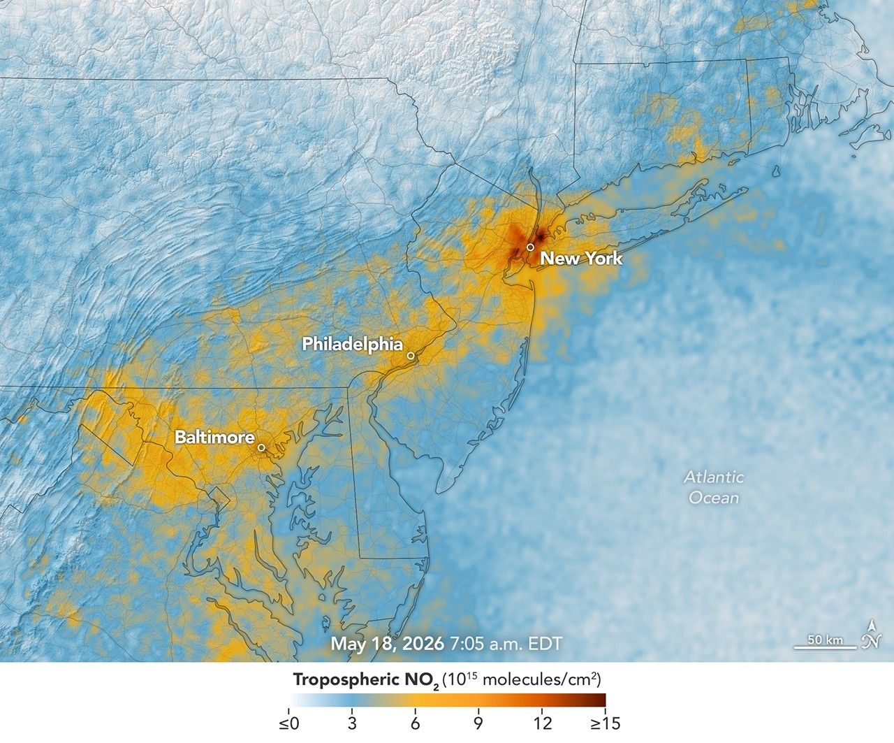


More than 35 million people live along the New York–Washington corridor and breathe the region’s air. While air quality has improved significantly in recent decades, outbreaks of ground-level ozone remain common, particularly in the warm summer months, when the chemical reactions that produce the pollutant accelerate and stagnant air allows ozone to accumulate.
A reminder of this seasonal phenomenon came earlier than usual in 2026, when a mid-May heat wave prompted the New York State Department of Health and the New York Department of Environmental Conservation to issue a health advisory on May 17 over concerns about ozone. The code orange advisory warned young people, older adults, and those working or exercising outdoors to limit activity due to ozone’s respiratory and cardiovascular health impacts.
As expected, ground-based air-quality sensors operated by state and federal agencies showed ozone reaching unhealthy levels for sensitive groups on May 18, something that typically happens several times per year. Meanwhile, NASA’s TEMPO (Tropospheric Emissions: Monitoring of Pollution) instrument observed the event from geostationary orbit 22,000 miles (35,000 kilometers) above the equator, a unique vantage point that allows the sensor to collect frequent observations of air pollution.
TEMPO detects nitrogen dioxide (NO2), a gas emitted by burning fuels, particularly by motor vehicles, that contributes to ozone formation. “There’s often a clear and interesting pattern in TEMPO’s nitrogen dioxide data during ozone alert days,” said Hazem Mahmoud, an atmospheric scientist at NASA’s Atmospheric Science Data Center at Langley Research Center. “We see high concentrations of nitrogen dioxide during the early morning commute that drop off sharply in the late afternoon as ozone increases.”
The decline occurs as sunlight fuels photochemical reactions involving nitrogen dioxide, volatile organic compounds, and oxygen that lead to ozone formation. By late afternoon, these reactions deplete much of the available nitrogen dioxide, slowing ozone production until the cycle begins again the next day.
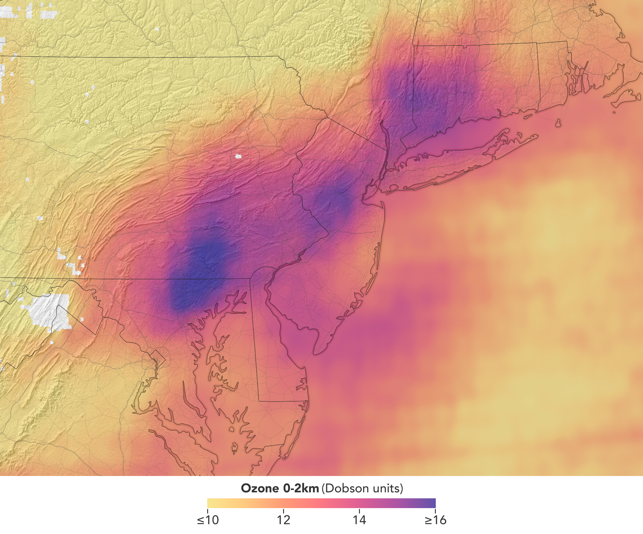
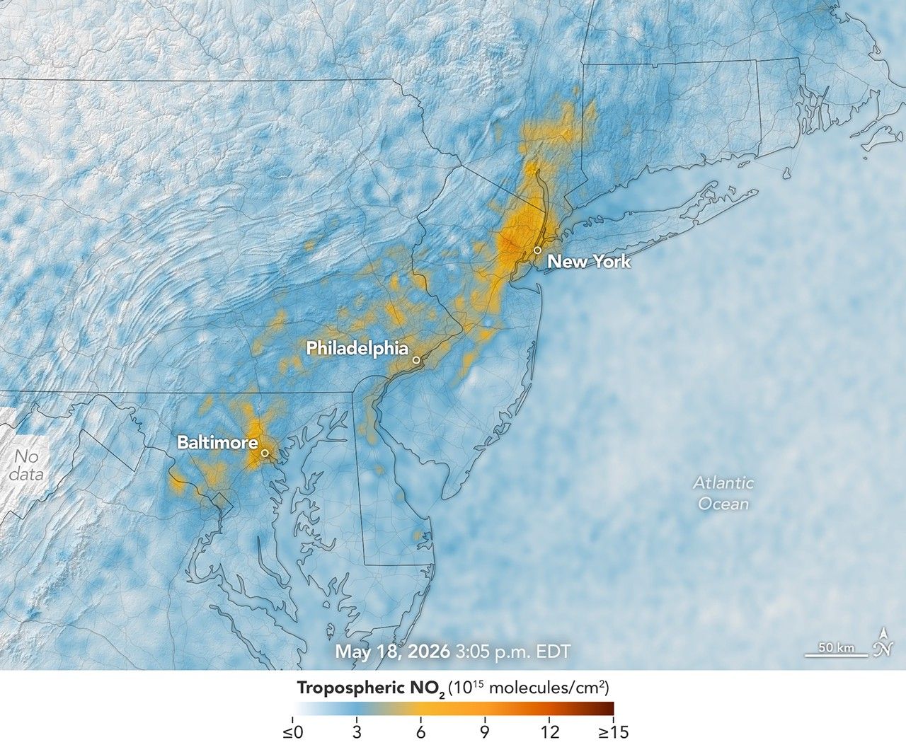
The pair of images above underscores the pattern. The image on the left was acquired at 7:05 a.m. local time when nitrogen dioxide concentrations were high during the morning commute. By 3:05 p.m. (right), most of the nitrogen dioxide had declined substantially, and surface ozone levels were elevated (below). Meanwhile, afternoon sea breezes appear to have transported the remaining nitrogen dioxide slightly to the west. Note that the data shown is provisional, and processing methods are still being refined.
Sensors on earlier polar-orbiting satellites, such as OMI (Ozone Monitoring Instrument) and TROPOMI (Tropospheric Monitoring Instrument), sampled nitrogen dioxide over New York once per day. After its launch in 2023, TEMPO began providing data every hour, allowing researchers to track the evolution and dispersion of air pollution at much finer time scales.
“TEMPO is helping fill data gaps between ground stations and allowing us to ask new questions,” Mahmoud said. The mission provides data that can improve not only air quality forecasts during crisis situations, such as wildfires, but also the atmospheric models used to forecast the daily rhythms of urban pollution. Such models help researchers understand how natural factors such as winds, humidity levels, and air temperatures influence pollution plumes over the course of a day.

TEMPO also detects ozone directly, but determining how much of that ozone is near the surface versus higher in the atmosphere can be challenging. Most of Earth’s ozone resides in the stratosphere, well above the troposphere, where people live and breathe. At times, however, stratospheric ozone can be transported downward into the troposphere. During events known as stratospheric intrusions, it can even descend far enough to affect air quality at the surface and add to the ozone produced at ground level.
By combining TEMPO observations with other sources of information, researchers are studying the processes that influence the distribution of ozone vertically in the atmosphere. On May 18, NASA’s ground-based tropospheric lidar network (TOLNet) in New York City recorded high concentrations of ozone near the surface, indicating that TEMPO was detecting mostly surface-level ozone associated with urban emissions and not ozone aloft, said Mahmoud.
However, on May 19, the same sensor observed a layer of ozone descending from above 5 kilometers (3 miles), he added, a clue that some of the ozone TEMPO detected that day may have originated in the stratosphere. “This is the type of information that leads to better air quality forecast models and more accurate alerts,” Mahmoud said. “Alerts can affect tens of millions of people and lead to disruptions in school, sports, and other activities, so it’s essential that they be as accurate as possible.”
On June 6, New York authorities issued another health advisory for ozone. People interested in following the event can access daily near-real-time TEMPO observations of ozone, nitrogen dioxide, and other gases on NASA’s Worldview browser, on an interactive Harvard & Smithsonian Center for Astrophysics browsing tool, and on NASA’s Earthdata portal.
NASA Earth Observatory images by Michala Garrison, using TEMPO data from NASA Earthdata. Story by Adam Voiland.


References & Resources
- Acker, S., et al. (2025) Satellite detection of NO2 distributions using TROPOMI and TEMPO and comparison with ground-based concentration measurements. Atmospheric Chemistry and Physics, 25(14), 8271-8288.
- City of New York (2024) Community Air Survey Report: 2008-2024. Accessed June 9, 2026.
- Energy Education, Ozone. Accessed June 10, 2026.
- Environmental Protection Agency (2026, May 13) What is Ozone? Accessed June 9, 2026.
- Environmental Protection Agency (2025, July 10) Basic Information about NO2. Accessed June 9, 2026.
- Holloway, T., et al. (2025) Satellite data to support air quality assessment and management. Journal of the Air & Waste Management Association, 75(6), 429-463.
- Lee, J., et al. (2024) The Evolutions and Large-Scale Mechanisms of Summer Stratospheric Ozone Intrusion Across Global Hotspots. JGR Atmospheres, 129(4),e2023JD039877.
- NASA (2026) TOLNet. Accessed June 9, 2026.
- NASA Air Quality (AQ) Monitoring from Space by NASA using TEMPO. Accessed June 9, 2026
- NASA Air Quality (2026) Nitrogen Dioxide. Accessed June 9, 2026.
- NASA Air Quality (2026) Nitrogen Dioxide Trends for US Cities. Accessed June 9, 2026.
- NASA Earthdata (2024, May 3) TEMPO Mission Releases Beta Level 1, 2, and 3 Version 03 Data Products. Accessed June 9, 2026.
- New York State Department of Environmental Conservation (2026, May 18) Air Quality Health Advisory Extended for New York City Metro Region. Accessed June 9, 2026.
- Zhang, J., et al. (2026) Revealing the Formation and Control of NYC Downwind Coastal High Ozone via New TEMPO Observations. Geophysical Research Letters, 53(2),e2025GL117523.
You may also be interested in:
Stay up-to-date with the latest content from NASA as we explore the universe and discover more about our home planet.

Seasonal fires have darkened skies over Southeast Asia.

As winter turned to spring, the skies over the Gulf of Alaska displayed textbook examples of numerous cloud formations.

Following a significant winter storm, frigid temperatures lingered in late January 2026 across a vast swath of the U.S.
Discover More from NASA Earth Science
Subscribe to Earth Observatory Newsletters
Subscribe to the Earth Observatory and get the Earth in your inbox.

Earth Observatory Image of the Day
NASA's Earth Observatory brings you the Earth, every day, with in-depth stories and stunning imagery.

Explore Earth Science
Earth Science Data
Open access to NASA’s archive of Earth science data
The post Air Pollution’s Daily Pulse Over the Northeast appeared first on NASA Science.