❌

Reading view

C V Raman: the physicist with a ‘Himalayan ego’ who went to Stockholm convinced he’d win a Nobel prize
C V Raman portrait
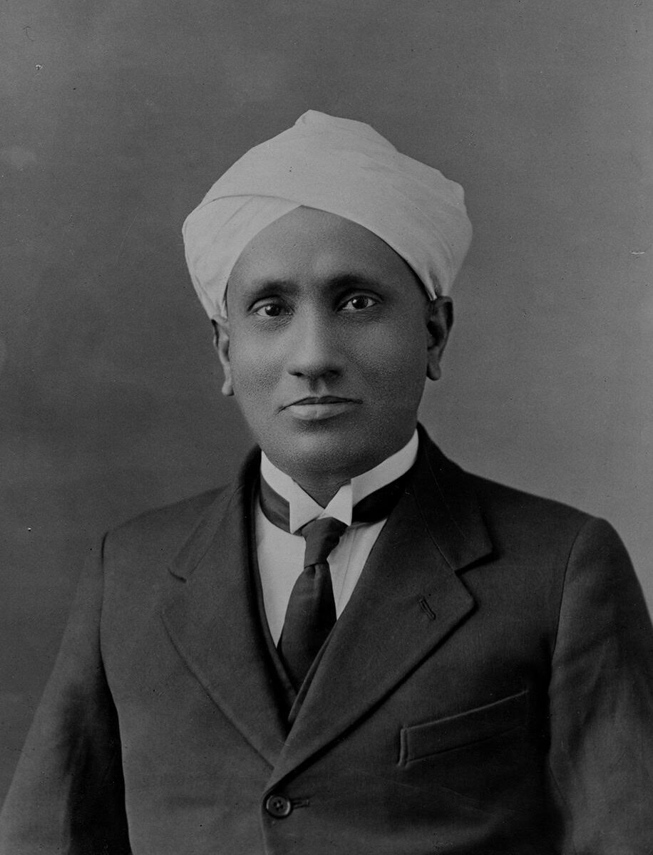
Cocksure and confident C V Raman sailed to Stockholm in 1930 convinced he’d win that year’s Nobel Prize in Physics. (Photograph by A Bortzells Tryckeri, courtesy of AIP Emilio Segrè Visual Archives, W F Meggers Gallery of Nobel Laureates Collection)

How confident, or perhaps delusional, do you have to be to travel to Stockholm because you’re so certain you’ll be awarded a Nobel prize? Most of us wouldn’t have the time, money or self-belief to go to Sweden and hang out at the Royal Swedish Academy of Sciences on the off-chance that we might win. But one person who did just that was the Indian physicist Chandrasekhara Venkata (C V) Raman in 1930.

Back in those days, travelling from India to Sweden wasn’t a case of jumping on a jet plane, but involved a long, two-month journey by sea. So if he wanted to arrive in Stockholm in time for the award ceremony on 10 December 1930, Raman knew he couldn’t wait until the prize was formally announced in mid-November to set sail. In July 1930 he therefore booked passage for himself and his wife, the couple arriving in Stockholm on 9 December of that year.

Raman’s audacity, belief and the arduous journey paid off. He was duly awarded the 1930 Nobel Prize in Physics “for his work on the scattering of light and for the discovery of the effect named after him”, namely Raman scattering. In doing so, Raman became the first person from India to win a scientific Nobel prize – the poet, playwright and musician Rabindranath Tagore having previously won the 1913 Nobel Prize in Literature.

Obsessive nature

Born on 7 November 1888  in the city of Thiruchchirappalli in Tamil Nadu, Raman was a child prodigy, who at 16 came top in physics at the University of Madras and published his first research paper aged just 18. Appointed a professor of physics at the University of Calcutta in 1913, Raman had a long obsession with winning a Nobel prize. In 1924, upon being elected a fellow of the Royal Society, he was asked during the award ceremony what was next in line for him. “The Nobel prize of course!” he replied.

The discovery that bagged Raman the coveted prize in fact began on another sea voyage

The discovery that bagged him the coveted prize in fact began on another sea voyage. In 1921 Raman was travelling back from Southampton to Bombay (now Mumbai) on the SS Narkunda, having taken part in the Second Congress of the Universities of the Empire in Oxford. Rather than lounging on the sun deck or drinking in the bar, Raman spent the 15-day journey examining and analysing the deep blue colours of the Mediterranean, Red and Arabian seas with his pocket Nicol prisms, a small telescope and a diffraction grating.

In fact, Raman did more than just take data. While on board, he wrote up his findings in a short letter that he mailed to the journal Nature while the ship was docked at Aden in Yemen. Published on 20 October 1921, it gives Raman’s address as “SS Narkunda, near Aden” (Nature 108 242). He then wrote another paper to Nature (108 367) titled “The colour of the sea”, this time with the byline “SS Narkunda, Bombay Harbour”.

The spectrum of blue colours of the vast sea fascinated Raman and made him question the previous belief, primarily from the work by Lord Rayleigh, that the colour is simply due to the reflection of the sky – and has nothing to do with the colour of the water itself. Raman challenged this notion in his follow-up Nature paper, which was published on 17 November 1921.

Mediterranean sea
Natural fascination C V Raman was awarded the 1930 Nobel Prize in Physics for discovering that light can change colour when passing through a material because some photons scatter inelastically off it. Now known as “Raman scattering”, he came up with the idea while sailing from the UK to India in 1921 and taking measurements of the deep blue colour of the sea. (Courtesy: iStock/Ciuvelic Razvan)

“It was abundantly clear from the observations,” he writes, “that the blue colour of the deep sea is a distinct phenomenon in itself.” Raman believed that light diffracts as it passes through the water and concluded: “An interesting possibility that should be considered is that the diffracting particles may, at least in part, be the molecules of the water themselves.”

This curiosity led him to a series of experiments over the next few years, primarily carried out by his students at Calcutta University, culminating in the discovery that light changes its wavelength and energy when it passes through any material. The change in wavelength and energy, in fact, is a fingerprint of the material itself.

His discovery of what became known as the Raman effect is what eventually won him his most cherished recognition – the 1930 Nobel Prize in Physics. One of the many applications of Raman’s discovery is Raman spectroscopy, which uses the scattering of laser light to establish the chemical make-up of a material and forms the basis of airport security scanners.

Indian impact

Raman’s Nobel prize was significant not just for the scientific advancements that his discovery enabled, but also for the far-reaching impact it engendered in India, where opposition to the British Raj was gathering speed. In fact, he won the award less than a year after the declaration of Purna Swaraj – complete independence – on 26 January 1930 in a session of the Indian National Congress in Lahore.

For a country reeling under colonial rule and fighting for its identity, Raman’s Nobel prize could not have come at a better time to instil hope and aspirations to millions of people around the country. In fact, he holds the honour of being the first physicist outside western Europe or the US to win the Nobel Prize in Physics.

C V Raman at 1930 Nobel ceremony
Dream trip C V Raman (far left) picking up the 1930 Nobel Prize in Physics in Stockholm alongside (from left to right) fellow winners Hans Fischer (chemistry), Karl Landsteiner (medicine) and Sinclair Lewis (literature). (No known copyright restrictions, photographer unknown. Source: Wikimedia Commons)

Raman was fully aware of the impact that the prize would have in India, where research was far less developed than that enjoyed by his counterparts in, say, Cambridge, Göttingen or Copenhagen. In 1929 he therefore hesitantly wrote a letter to the Danish Nobel-prize-winner Niels Bohr, asking for his “influential support” for the 1930 Nobel prize. The request of such “personal character”, he explained, was only because he believed that Bohr would “sympathize with the scientific aspirations of India”.

Unbeknownst to Raman, Bohr had already nominated him for a Nobel prize in 1929 – that year’s prize going to Louis de Broglie for wave–particle duality – and he did so again in 1930. We now know a total of 10 different people nominated Raman for that year’s prize, including de Broglie as well as Ernest Rutherford and Charles Wilson.

Raman’s research and notoriety led to many students being attracted to Calcutta, with the physics department becoming a centre of world-class research

Raman’s research and notoriety led to many students being attracted to Calcutta (now Kolkata), with the physics department becoming a centre of world-class research despite its small size and the lack of an established scientific culture and infrastructure in India. Other leading physicists to have worked there include the astrophysicist Meghnad Saha and the theorist Satyendra Nath Bose in what some have touted as a “golden era” for Indian science.

Sadly, it ended prematurely a few years after Raman’s Nobel prize due to conflicts between these three leading scientists. This was partly due to parochialism and partly, as his biographer, the condensed-matter physicist Ganeshan Venkataraman famously put it, Raman’s “Himalayan ego and sharp tongue”.

Moving on

In 1933 Raman left Calcutta, becoming the first Indian director of the Indian Institute of Science (IISc, earlier the Tata Institute of Science) in Bangalore (now Bengaluru). Rutherford, when asked by the institute’s council as to who should replace the outgoing director Martin Forster, had made it clear there was no need to seek directors in Britain when India had a “distinguished candidate in the shape of Raman”.
Formal portrait of Gamow, Bohr, Raman, Klein, Lauritsen, Rasmussen
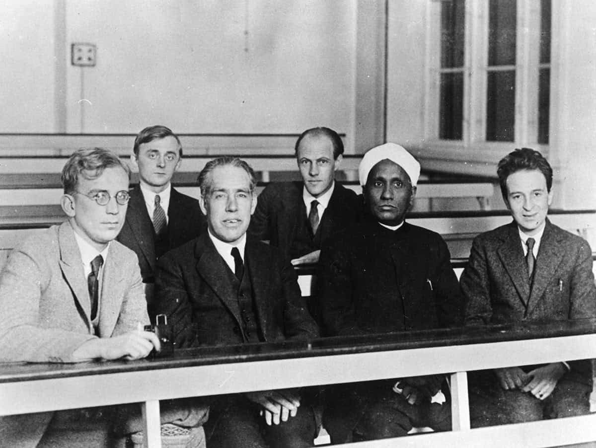
Mixing of minds C V Raman (second right) personally wrote to Niels Bohr (second left) for his support for the 1930 Nobel prize. The pair are shown here at the Niels Bohr Institute, Copenhagen, alongside George Gamow (far left) and Oskar Klein (far right) and Charles (back row, left) and Ebbe Rasmussen (back row, right). (Courtesy: AIP Emilio Segrè Visual Archives, Margrethe Bohr Collection)

In 1934 he went on to found the Indian Academy of Science, which was significant in that it provided a way for researchers across the country to communicate and discuss research findings. Just as important, however, was the fact that membership of the academy was reserved exclusively for Indian scientists, effectively signalling an act of rebellion against the British.

Raman’s time at the IISc was controversial. On one occasion, he turned down the application for a research fellowship by a female student – the biochemist Kamala Sohonie – because he believed women were not competent to conduct research. Raman reversed his decision, albeit with humiliating conditions, after Sohonie staged a Gandhian-style protest (Satyagraha) outside his office.

Within three years, Raman was forced to resign from the directorship following a fallout with the council, primarily for allegations of bias towards physics research and overshadowing other areas of research of the institute. He remained a professor at the IISc until retiring in 1948. Later that year, he founded the Raman Research Institute with which he was actively involved until his death in 1970 at the age of 82.

Raman’s legacy

Despite his controversial past, Raman is still the flag-bearer of Indian physics, owing to the Nobel prize and the global recognition he enjoyed. India holds a National Science Day every year on 28 February to mark the occasion in 1928 when Raman and his associate Kariamanickam Srinivasa Krishnan announced their discovery of Raman scattering to the media. The work was reported in newspapers on 29 February and was formally published on 31 March 1928 in a paper entitled “A new type of secondary radiation” (Nature 121 502 ).

Almost a century on from his success, however, India has not yet produced another home-grown Nobel-prize-winning physicist. Raman’s nephew Subrahmanyan Chandrasekhar did share the 1983 Nobel Prize in Physics with William Fowler for his work on the evolution of stars, but he was based in the UK and then the US when the work for which he was recognized was carried out.

Raman’s divisive personality and sharp opinions turned more people against him than his ingenuity and scientific legacy ever won over

Sadly, Raman’s divisive personality and sharp opinions turned more people against him than his ingenuity and scientific legacy ever won over. His obsession with global recognition can be sensed from his reaction upon first receiving news of his Nobel prize, which came while he was en route to Stockholm. Learning of the award from his Calcutta collaborator Suri Bhagavantam, Raman’s first reaction was to ask if he was the sole awardee or whether he was to “share the bed with other strangers”.

Given his “Himalayan ego”, it should perhaps come as no surprise that Raman decided to travel to Stockholm on a whim. We do not have any documentation about what he thought or did on that two-month voyage. But for him, at least, it was a journey that was not wasted.

SmarAct Group logo

SmarAct proudly supports Physics World‘s Nobel Prize coverage, advancing breakthroughs in science and technology through high-precision positioning, metrology and automation. Discover how SmarAct shapes the future of innovation at smaract.com.

The post C V Raman: the physicist with a ‘Himalayan ego’ who went to Stockholm convinced he’d win a Nobel prize appeared first on Physics World.
  •  

Mercury may not need an ancient dynamo to explain its magnetic crust

A new study using data from a space mission suggests that most of Mercury’s crustal magnetic fields can be explained by iron and other magnetized rocks in the crust responding to the planet’s weak present-day core magnetic field, rather than from an ancient field, as had been inferred previously. Mercury is the only solar-system planet other than Earth to possess both a global magnetic field arising from its core and a crustal magnetic field resulting from rocks that were magnetized in either the present-day or an ancient core field. Present-day (induced) magnetization reveals the location and amount of iron in the crust, whereas ancient (remanent) magnetization records the planet’s dynamo history.

NASA’s MErcury, Surface, Space ENvironment, GEochemistry and Ranging (MESSENGER) mission observed the planet in 2011–2015. Data from the mission are allowing scientists to explore the strength and distribution of Mercury’s magnetic field. During the mission, a last-minute decision was made “to reduce the orbit altitude thereby allowing crustal fields to be detected” explains Lon Hood at the Lunar and Planetary Laboratory at the University of Arizona. He has worked extensively on Mercury’s crustal magnetism using the MESSENGER data but was not involved in the new study.

Crustal magnetism was expected to be “partly due to remanent magnetization dating from the time when the crustal sources formed in the planetary magnetic field,” Hood says. This interpretation is drawn from earlier analyses of the mission data. But a key challenge in understanding the crustal magnetic field remained – how to delineate the contributions of induced and remanent magnetization. Separating the relative contributions of ancient and present-day induced magnetization on the crustal magnetic field can reveal new ways of understanding the spatial abundance of magnetic rocks, variations of magnetic properties of crustal minerals, and the dynamo history of Mercury.

New insights from old data

The new study, led by Catherine Johnson at the University of British Columbia in Vancouver, uses field observations of Mercury’s crustal magnetic fields from MESSENGER to develop a magnetization model of the planet and identify sources of its magnetization. The researchers calculated the expected induced magnetization strength using the low-altitude observations with assumptions on the crustal thickness, magnetic mineralogy, iron content, and the present-day core field.

In line with previous studies, the researchers found that the largest magnetization strengths occur in the Caloris region, along with localized signals elsewhere. The spatial pattern of magnetization strength, however, does not consistently match the variation in near-surface iron content seen in MESSENGER spectroscopic data. Instead, magnetization strength correlates with crustal thickness, up to about 30 km, suggesting the magnetized rocks are concentrated within the upper part of the crust.

The researchers found that induced magnetization is relatively small, given the low iron content of the planet’s crust and its weak core field – about a hundred times weaker than Earth’s. Even so, they estimate that induced magnetization can fully account for the calculated magnetization strength across more than 85% of the area north of 38 °N. This assumes it extends through the crustal column to a depth of about 30 km, which means that no remanent magnetization is required to explain the observed crustal field over that majority of the mapped region. Areas where induced magnetization does not explain the observed crustal fields may be the result of iron delivered by ancient asteroid impacts, which would locally increase the induced magnetization. Elsewhere, a contribution from remanent magnetization may be required to explain the observed fields.

Towards better characterization

On Earth, the robust separation of induced and remanent magnetizations requires laboratory measurements of rock samples. For Mercury no such samples exist, so the magnetic properties of its crust must be inferred from satellite observations constrained by assumptions about the composition and magnetic behaviour of its rocks. The delineation in the new study depends on “assumptions about magnetic mineralogy that cannot be verified due to the lack of returned samples”, says Hood.

Better characterization of the crust’s low-field magnetic susceptibility – currently inferred from a limited number of laboratory measurements on meteorites and minerals believed to resemble Mercury’s crust – can advance our understanding of Mercury’s crustal fields. Better core-field models and higher-resolution iron maps from the European–Japanese BepiColombo mission could help. This mission comprises two spacecraft that launched in 2018 and is expected to run until 2029.

However, Hood says “there are no current plans for either spacecraft to approach near enough to the planet to detect or map more of the crustal magnetic field”. Although the spacecraft will eventually descend below 100 kilometres, giving us a first look at the southern hemisphere. Indeed, we may have a long wait before we have the complete picture because Hoods says, ” there are no plans to obtain samples of Mercury’s crustal rocks, which are needed to definitively determine the origin of the crustal magnetization”.

The researchers report their findings in PNAS.

The post Mercury may not need an ancient dynamo to explain its magnetic crust appeared first on Physics World.

  •  

Earthquake fault irregularities control rupture speed and influence ground motion

Earthquakes that propagate at higher speeds make the ground move more than it would in slower but otherwise comparable earthquakes, say geophysicists. Using physics-based models, Mohamed Abdelmeguid and colleagues at the California Institute of Technology in the US showed that so-called “supershear” ruptures produce stronger and longer-duration ground motion than equivalent subshear ruptures. Because models of ground motion that underpin infrastructure standards do not account for this effect, these models may need to be updated to accurately describe hazards such as the 2025 Myanmar earthquake, which produced supershear ruptures in both directions.

Geophysicists have identified two categories of earthquake based on how fast their ruptures propagate through the Earth’s crust. Shear waves, or S waves, travel at certain expected velocities (the shear-wave velocity) depending on the stiffness and density of the ground. When a rupture travels faster than the shear-wave velocity of the surrounding ground, it is termed a supershear earthquake. Otherwise, it is subshear.

Although Abdelmeguid notes that supershear ruptures were first predicted theoretically in the 1970s, and have subsequently been observed in both laboratory experiments and the real world, most previous studies focused on their underlying mechanisms and the transition from subshear to supershear. The new study, which appears in the Bulletin of the Seismological Society of America, goes a step further by examining how the ground motion in a supershear quake differs from that of an otherwise comparable subshear one. The question is relevant, Abdelmeguid says, because nearly 36% of strike-slip earthquakes during the past 15 years contained supershear rupture, yet existing models do not factor it in.

Supershear simulations

To address this gap, Abdelmeguid and colleagues developed a dynamic rupture model that generates simulated ground motion data and used it to identify the characteristics of supershear earthquakes. They found that prolonged supershear propagation produces what they term “a distinct spatial pattern of stronger and longer-duration shaking”. However, episodic supershear segments, where rupture speed intermittently changes between supershear and subshear, produce ground motion similar to subshear ruptures.

Simulations like these are important because some supershear rupture scenarios are poorly represented in the observational record. This record is used to develop ground motion models, so simulations can “reveal physical dependencies that may not be apparent from existing observations,” Abdelmeguid says.

Characterizing the 2025 Myanmar earthquake

The 2025 Myanmar earthquake – a supershear quake in which many regions experienced higher than expected ground shaking – is a case in point. It occurred on the 1200-kilometre-long Sagaing Fault, which lies at the boundary of the Burma microplate and the Sunda plate and is not far from Mandalay, the country’s second-largest city. At magnitude 7.7, it was the largest earthquake in Myanmar in over a century, and the long rupture meant that large parts of Myanmar and Thailand were affected, with thousands of deaths and injuries as well as severe damage to infrastructure.

Initial studies were inconclusive about whether this earthquake’s rupture exhibited intermittent or sustained supershear speed. This lack of consensus is partly because recording intermittent supershear rupture is challenging when near-fault sensors are sparse, as is the case in Myanmar (and indeed most countries, with notable exceptions such as Japan, Taiwan, New Zealand and parts of the US).

A new study published in PNAS addresses this question. Using satellite earth observations, teleseismic data and CCTV footage as well as the available near-fault seismic sensor data, researchers led by Lingling Ye at the Southern University of Science and Technology (SUSTech) in China modelled the rupture process of the Myanmar quake. The result, Ye says, is a “well-resolved rupture process” that “reveals previously unrecognized dynamic rupture features”. Notably, the team’s simulations showed that the rupture transitioned between supershear and subshear as it tore through around 460 kilometres of the country.

Influence of geometry and stress distribution

To understand the cause of these variations, the researchers examined the geometry and stress distribution along the fault. Based on an existing fault model, they calculated a parameter called fault misalignment, which acts as an indicator for irregularities in the fault geometry. Higher fault misalignment, for example, indicates higher bends and branches in the fault.

When the researchers overlaid fault misalignment with the observed rupture speed, they noticed that supershear speeds coincided with fault stretches that had lower misalignment. For fault stretches with higher misalignment, subshear speed prevailed, meaning that the rupture decelerates at locations with high fault misalignment, transitioning from supershear to subshear. The researchers also found that the rupture speed, whether supershear or subshear, responded to the varying levels of local stress, with higher stress levels inducing faster rupture speed.

Although not unique in exhibiting supershear behaviour, the 2025 Myanmar earthquake rupture propagated away from the epicentre on both sides, travelling around 80 kilometres to the north and 380 kilometres to the south. Initial studies debated whether the ruptures on both sides were supershear. The researchers found that the northern rupture propagation was not supershear and claim that its shorter rupture length is caused by a combination of the fault’s complex structure and low accumulated stress resulting from the magnitude 6.8 earthquake that struck in 2012.

“Every earthquake has unique behaviour”

In future work, Ye is eager to revisit the 2023 Turkey doublet earthquakes, which she says have many more near-fault strong motion observations than the 2025 Myanmar quake, as well as a now well characterized complex fault system. “Every earthquake has unique behaviour,” she says. “Determining the key features that control their rupture processes is still underway.”

For Abdelmeguid, who recently started his own research group at the University of Houston, US, understanding these complex rupture processes is important because it will ultimately improve our understanding of geophysical processes and the ground motion models that are used for engineering applications. “We are currently extending this work to examine ground motions generated by ruptures on more complex faults, including cases in which fault geometry and heterogeneity influence both ground motion and the dynamic process, as observed during the multiple earthquakes,” he tells Physics World.

  • This article was amended on 2 September 2026 to clarify the nature of the rupture propagation in the 2025 Myanmar earthquake. The researchers found that the northern rupture was subshear, not supershear as originally stated.

The post Earthquake fault irregularities control rupture speed and influence ground motion appeared first on Physics World.

  •  

Physics-based simulations could improve earthquake-damage predictions, why aren’t they being used?

Earthquake ground-motion predictions rely on statistical models built on historical records. This means that ground-motion measurements taken during previous earthquakes are used to predict the effects of future earthquakes. However, historical data can be sparse in some locations and if a region has not experienced a severe earthquake in the modern era, there will be no data for high-magnitude events. As a result, seismologists are keen on using physics-based simulations to predict ground motions, essentially filling in the gaps in historical datasets.

Although physics-based simulations of ground motions have been in development for while, they have rarely been used for engineering applications or building code development. With advancing computational capacities and geophysical understanding of earthquake cycles, the development and application of physics-based simulations have seen a surge of energy in the last few years.

As someone working with physics-based ground motions and enthusiastic about the latest research in the field, I arrived in Portland, Oregon in July for the quadrennial US National Conference on Earthquake Engineering (NCEE) hosted by the Earthquake Engineering Research Institute. This was my third NCEE – I was about to start my PhD when I attended the first time in 2018 in Los Angeles.

After a series of delays during my flight from London, I finally arrived in Portland in the quiet hours of the night. Only realising that I had about six hours before the first session starts in the morning.

Understanding the challenges

Regardless, I reached the venue at 9 am sharp, the Oregon Convention Center, with swollen (and perhaps red) eyes, to attend a workshop on “Earthquake ground motion simulation validation & utilization for engineering applications”. I was keen to understand why the validation and application of simulated ground motions are still challenging despite advancements in research and tools for simulations. A little sleep deprivation through jetlag did not deter me.

Current ground-motion models are used within a probabilistic framework, along with models of the fault systems and the earthquake magnitudes they can generate, to define probabilities of expected ground shaking. These statistical models do not capture the geophysical process but instead rely on a curated dataset collected in the short history of earthquake recordings. These datasets, likely, do not contain all possible earthquake magnitudes and ground shaking. Models based on these data are prone to bias, especially for scenarios where data are sparse. For example, the data gap is stark for higher magnitudes at shorter distances from the source, since we have only seen a handful of large earthquakes after earthquake recording started in the last century.

Physics-based simulations can meaningfully augment these datasets, and in turn, improve conventional ground motion models. Many such efforts have been made globally in the past decade. My PhD research deals with built environment impacts from a simulated magnitude 9 Cascadia subduction zone, which runs hundreds of kilometres along the coast of the Pacific Northwest of the US and southwestern Canada. Indeed, the subduction zone is about 200 kilometres west of where the conference was happening. Although this fault has never produced a magnitude 9 earthquake, or any significant earthquake, in the last century, there is geological evidence of several large magnitude earthquakes over a period of thousands of years.

“Different answers”

My research involved understanding how the built environment would be impacted by such a large earthquake on this fault. That research, and many others, showed that we can gain nuanced understanding of how ground shakes, impacts the built environment and cascades into landslides and tsunamis after an earthquake. As Stanford University’s Greg Deierlein, said during the workshop, “Simulations are most useful when they provide different answers compared to conventional methods.”

Despite their promise, physics-based simulations remain unused in most national seismic hazard models. And where they are used, the scale is negligible. The ingredient that is missing is trust – whether the simulations can represent complex fault geometry and rupture mechanism, how reliable are the velocity structure models, can the simulations reproduce empirical data. Trust, within the community of researchers and practitioners, is built on testing and validation.

Aptly, there was engaging discussions during the workshop around standardized validation protocols and open repositories of reproducible workflows. One key challenge for physics-based simulations is to establish that simulated ground shaking scales across various parameters in patterns that is empirically observed in the recordings. As Jonathan Stewart at the University of California Los Angeles, pointed out, “the trust on absolute amplitude [from physics-based simulations] is low, however, how does the [simulated] ground motion scale across various parameters is what is valuable.”

There was at least one session each day discussing methods of developing, validating, and applying physics-based simulation of ground motions. I presented my work on the final session, a closing act if you will, on using the simulated ground motions to reveal damage patterns across a building portfolio that conventional ground motion models cannot capture. It implies that we may have two very different views of risk depending on which models we use. This would make it challenging for insurance companies to correctly price the risk and for future infrastructure developments in the region.

With more encouragement and more questions than answers, I wrapped up five long-days of exchanging ideas, discussing careers, and catching-up with friends. While walking past beautiful murals and aisles of books in Powell’s Books on my last evening in Portland, I wondered how far simulated ground motions will travel by the time I come back for the next NCEE four years from now.

The post Physics-based simulations could improve earthquake-damage predictions, why aren’t they being used? appeared first on Physics World.

  •  

Earthquake sensors reveal vital information about how hurricanes move and grow

Sensors designed to record earthquakes can reveal insights into a very different natural hazard – how hurricanes evolve and intensify as they strike land. The surprising connection has been made by researchers in the US, who examined data from seismic sensors installed in Louisiana for studying the interior of the Earth. They found that the sensors, which collected data on pressure fluctuations, provided information about how Hurricane Isaac grew and intensified as it struck and devastated the state in 2012.

Earthquakes and hurricanes are very different in how they form, move and impact the Earth. The parameters governing these natural hazards – and the way that we measure them – are also distinct given that one is a geophysical phenomenon and the other atmospheric.

Hurricanes, which form over warmer tropical and subtropical ocean waters, are rotating systems of cloud and thunderstorms. They consist of a calm, central “eye”, a surrounding layer of tall thunderstorms, and strong winds called the “eyewall”. Spiralling away from the eyewall are bands of clouds and thunderstorms.

Forecasters describe the structure and evolution of hurricanes using three main parameters: track, intensity and the radii of the wind layers around the eye. But when hurricanes strike land, particularly important is the turbulence in the lowermost layer. That’s where momentum, heat and moisture mix between the atmosphere and the ocean or land.

Eyeing up hurricane path and intensity

Measuring the turbulence in this boundary layer is critical both for forecasting wind intensity and for developing and validating weather models. Such data are usually collected using reconnaissance aircraft, ocean buoys and onshore towers and radar. But flying planes into hurricanes is dangerous, while onshore towers are sparse, making data-gathering tricky. Continuous monitoring of a storm’s passage is not easy either.

In the new study, Qing Ji, Ipshita Dey and Eric Dunham from Stanford University processed data from seismic stations in Louisiana that are part of a network of 1700 stations across the US. Equipped with both infrasound sensors and seismometers, these “seismoacoustic” stations are designed to record seismic activity.

The infrasound sensors measure pressure fluctuations at the Earth’s surface, with the seismometers recording the resulting elastic response. But when the hurricane passed through the equipment, the winds were strong enough to leave an additional signal. In fact, the Stanford team found that the data revealed the calm eye and the turbulent eyewall – as well as the circular layers of thunderstorms and winds as the hurricane passed through the sensors.

“The infrasound sensors provide direct measurements of turbulent pressure fluctuations,” says Dunham. “We also used the seismometer data together with data from other atmospheric sensors to calibrate a computer model of hurricane turbulence.” The model provided space-time correlations of pressure fluctuations around the station, while the simulated pressure spectra matched the recorded data at station.

The researchers then calculated the Earth’s elastic response using the simulated pressure field, which aligned with the observed vertical displacement. More importantly, the simulations showed that the relevant parameter for calculating the Earth’s elastic response to pressure fluctuations is the velocity at which those fluctuations are carried downstream — rather than the near-surface wind speed as had been assumed.

Exploiting existing sensor networks

Dunham told Physics World that he hopes the study will draw attention to the potential of seismoacoustic networks for atmospheric sciences. “Perhaps this will lead to deployments of seismometers and infrasound sensors in areas where coverage is currently sparse, like in the southeastern US,” he adds.

Those hopes are echoed by Ji – now based at the University of Texas, Austin – who says there is a growing interest in the use of these “noise” signals for environmental monitoring. As Ji points out, the beauty of seismic stations is that they record data continuously and have a high sampling rate compared to other sensors.

Seismoacoustic stations have already been used to study various environmental and climatic phenomena, such as rising amounts of energy in ocean waves as waters warm and the evolution of tropical storms and accompanying winds. “The atmospheric imprints, however, are less studied partly due to the overall smaller amplitudes and the potentially more complicated nature,” Ji adds.

Dunham also sees an opportunity to add infrasound sensors and barometers, both of which measure atmospheric pressure, to existing seismometers. “Having multiple sensors at a single location opens up new opportunities for studying both the solid Earth and atmosphere,” he says.

The researchers report their findings in Science.

The post Earthquake sensors reveal vital information about how hurricanes move and grow appeared first on Physics World.

  •  

Seismic waves reflected from Earth’s core moved parts of Japan 5 mm east

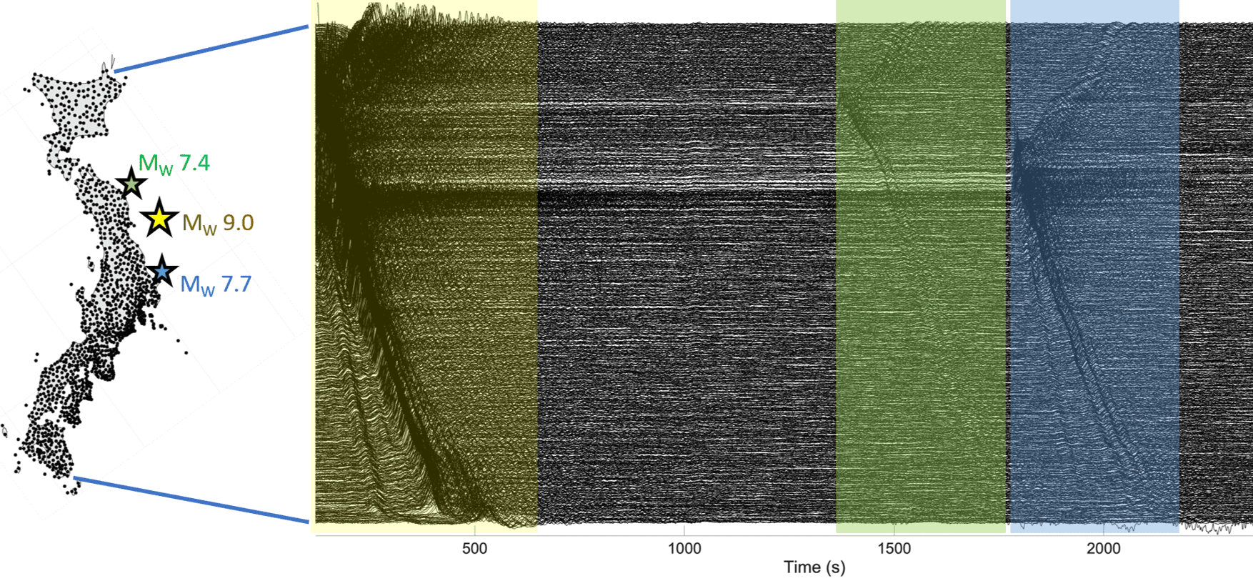
(left) A map of Japan densely covered with dots. Three stars off its eastern coast show the locations of the epicentres. (right) Graph showing eastward components of ground motion at each site. The graph resembles a bunched-up sheet, with the biggest bunches associated with the main quake (a period of up to ~600 s shown in yellow) and the two aftershocks shown in green and blue at 1500s and 2000s respectively.
Shifting eastward (left) A map of Japan showing the epicentres of the main shock (Mw 9.0) and two strongest aftershocks (Mw 7.7 and 7.4) in the Tohoku-Oki earthquake. Each black dot represents a GNSS station. (right) The observed eastward components of ground motion at each of the GNSS sites from northeast (top) to southwest (bottom) of Japan are shown in black traces, with the shaded areas representing ground motion corresponding to the main shock and the aftershocks. (Courtesy: Sunyoung Park; motion data from P Xu et al. Earth, Planets and Space 71 43 2019)

A previously unrecognized source of seismic hazard caused parts of Japan to move eastwards by up to 5 mm within minutes of the 2011 Tohoku-Oki earthquake. Conventionally, such shifts occur when seismic waves generated by rupturing tectonic plates cause the plates to slip, triggering movements of the land mass and the ocean floor. But a new study finds that in the Tohoku-Oki quake, the real culprit was waves that travelled down to Earth’s core and back – a phenomenon more usually associated with efforts to image structures deep inside the Earth.

The 2011 Tohoku-Oki quake occurred at the boundary between the Pacific plate and the North American plate, with an offshore epicentre around 130 kilometres east of Sendai. At magnitude 9, it was one of the largest recorded earthquakes in history, and it caused widespread devastation, including thousands of fatalities. The tsunami that followed exacerbated this damage, with meltdowns of three out of six nuclear reactors at the Fukushima Daiichi power station releasing radioactive caesium into the air and water and prompting a large-scale evacuation with long-term health impacts.

The earthquake was bigger than most models estimated, which compelled seismologists to examine and revise existing models of the largest possible earthquakes and their frequencies in the boundaries of tectonic plates. Instrumented records of this earthquake are still revealing new information about geophysical processes in the boundaries of tectonic plates.

Surface to core and back

In the new work, researchers led by Sunyoung Park at the University of Chicago, US studied shear waves recorded following the earthquake in Japan’s dense network of high-rate Global Navigation Satellite System instruments. Along with the expected seismic waves from the earthquake rupture, the team found so-called ScS waves that travelled thousands of kilometres through the Earth, bounced off the core and travelled back to the surface, arriving across Japan almost simultaneously 13 minutes after the main shock. “The name ScS reflects that path: S[hear] through the mantle, c for reflection at the core-mantle boundary, and then S again on the return path,” Park explains.

Although seismologists have studied ScS waves extensively, they have mostly done so for the purpose of imaging the deep Earth. “Because [ScS waves] reflect from the core-mantle boundary, they have helped constrain the depth and properties of the core-mantle boundary; the structure of the lowermost mantle; attenuation and anisotropy in the mantle; and source characteristics of large earthquakes,” Park explains.

The team’s study offers the first evidence that ScS waves can also trigger significant displacement-causing slip after an earthquake, meaning that earthquake hazard researchers may need to consider these waves to fully capture consequences of earthquake ruptures on the land as well as deep within tectonic plates.

A high-quality, high-resolution dataset

Two aspects of the Tohoku-Oki earthquake made it an incredible opportunity to study the role of ScS waves in triggering a slip event. The first is the nature of the earthquake itself. As well as releasing tremendous amounts of energy, it occurred on a shallow tectonic fault that is dipping down. This combination sent strong shear wave energy travelling nearly vertically down to the core, generating ScS waves strong enough to trigger movement in the tectonic plates.

The second was the quality and resolution of data. “Because Japan is so densely instrumented, we can look for small, coherent signals that would likely be invisible elsewhere,” Park says. “This made it a natural case in which to ask whether delayed seismic phases might trigger additional deformation.”

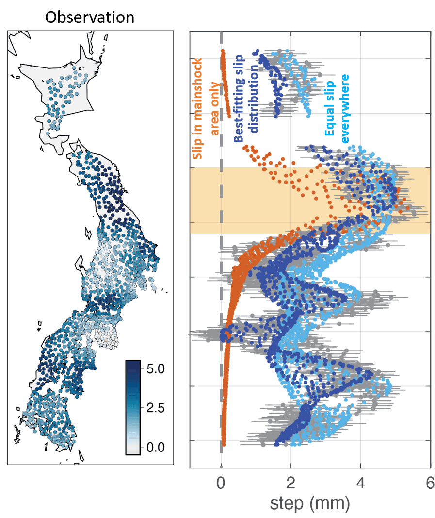
Working with Hiroo Kanamori at the California Institute of Technology (Caltech), US, and Luis Rivera at the University of Strasbourg, France, Park considered whether Earth’s elastic response to the main shock could explain Japan’s 5-mm displacement. To better understand this possibility, they calculated displacements at all the instrumented locations for many possible configurations of the earthquake rupture. However, the results did not reproduce the observed eastward motion.

At left, a map of Japan covered with dots in different shades of blue, with lightest blue representing no displacement and the darkest blue representing 5mm displacement. Large areas of Japan, especially the northeast, are dotted in dark blue. At right, a set of orange, dark blue and light blue dots representing the results of different models of displacement. The simulated data for equal slip everywhere fits the observed data better than the data for slip in main shock area only.
Competing models (left) Observed displacements in mm shown with coloured dots at each GNSS site across Japan. (right) The calculated displacement that would have occurred for slip only in the main shock area (orange dots), equal slip across the tectonic plates (light blue dots) and best fit slips corresponding to the observed displacement (dark blue dots). (Courtesy: Sunyoung Park)

The researchers then simulated possible slip scenarios across the tectonic plate interfaces, hoping to better characterize the levels and spatial extent of the slip that caused the eastward displacement. “The inferred slip event likely involved interfaces where the Pacific plate subducts beneath the Okhotsk Plate, and where the Philippine Sea plate subducts beneath the Eurasian plate,” Park says. Exactly how far this slip propagated, however, is still unknown because of the paucity of instrumented locations beyond Japan.

A slow-motion slip

Although the most memorable earthquakes and tsunamis are the ones that manifest havoc on Earth’s surface, the tectonic plates underneath are in perpetual but slow motion. At higher depths, these slow-moving plates produce earthquake events that unfold over days or weeks. Such events are called slow-slip or silent earthquakes and are important for accumulating and releasing stress as part of the earthquake cycle.

Rather than triggering a fast earthquake rupture, the ScS waves from the Tohoku-Oki quake appear to have set off a slow slip event spread over a very large area at intermediate depths of 20–60 km. This is the depth range where seismologists commonly observe silent earthquakes, and it provides avenues for understanding the dynamic processes that impact the earthquake cycle. This continuous flux in Earth’s deeper layers is a source of curiosity for many seismologists, including Park.

“A broader motivation for me is a general interest in deep-shallow interaction in the Earth,” Park tells Physics World. “I am especially interested in cases where processes or wave propagation involving the deep interior can influence faulting and deformation in the shallow lithosphere or vice versa.”

The researchers report their findings in Science.

The post Seismic waves reflected from Earth’s core moved parts of Japan 5 mm east appeared first on Physics World.

  •  
❌