❌

Normal view

Seeking Technosignatures in Polluted White Dwarfs

15 July 2026 at 17:00

white dwarf with debris disk

White dwarfs often show signs of metals in their spectra, providing evidence that these evolved stars have accreted planetary material. Could white dwarf spectra also provide evidence for technological activity in these star systems?

A Record of Planets Past

When a Sun-like star reaches the end of its hydrogen-burning lifetime, it first puffs up into a red giant before exposing its white-hot core, which evolves into a white dwarf. This dramatic transition shakes up any planets that happened to be orbiting the star, and some close-in planets may end up crumbling apart, their rubbly remains peppering the surface of the white dwarf.

So far, astronomers have found hundreds of white dwarfs that appear to be polluted with heavy elements from their destroyed planets. These observations provide a valuable look into the bulk compositions of planetary materials outside our solar system. They may also provide a way to detect patterns of chemical abundances that are not natural, resulting from technological processes like industrial refining or the creation of alloys — in other words, a technosignature that is evidence of not just life, but technologically advanced life.

Seeking Signs of Technology

abundances of meteorites compared to white dwarfs

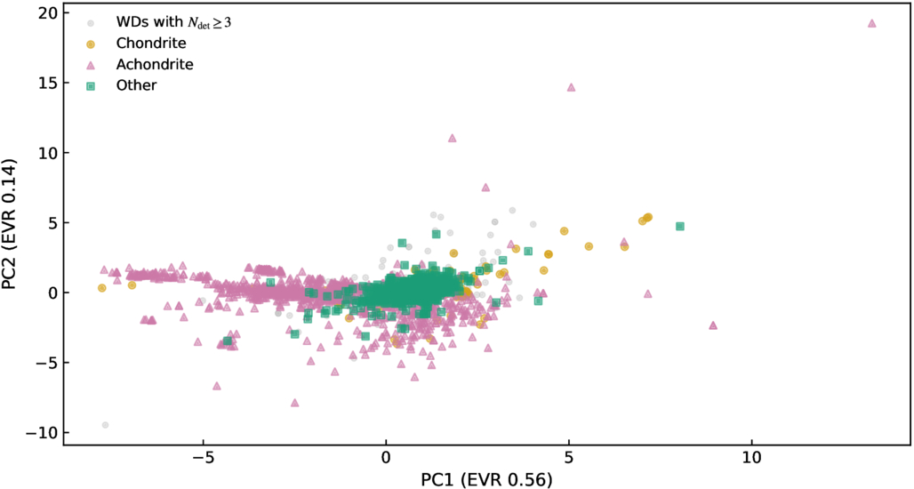
Representation of the chemical abundances of meteorites (pink, orange, and green) and white dwarfs (gray). Most white dwarf abundances overlap with the parameter space defined by the meteorite sample. Click to enlarge. [Huang et al. 2026]

A team led by Bo-Lun Huang (黄博伦) from Beijing Normal University recently investigated whether there is evidence for chemical technosignatures in the current sample of polluted white dwarfs. Huang and collaborators began their investigation with a catalog containing 697 measurements of white dwarfs with metals in their spectra. They applied Bayesian statistical methods to weigh the hypothesis that the chemical makeup of these white dwarfs is entirely natural against the possibility that they contain a blend of natural and technologically altered material.

The team used thousands of chemical abundance measurements from meteorites as a reference for the natural bulk composition of planetary material. For the mixture of natural and processed material, they combined the meteorite reference material with a template that is metal-rich and silicate-poor, with enhanced amounts of iron, nickel, chromium, and manganese.

plot showing evidence for a natural + processed model relative to a natural model as a function of the number of elements detected

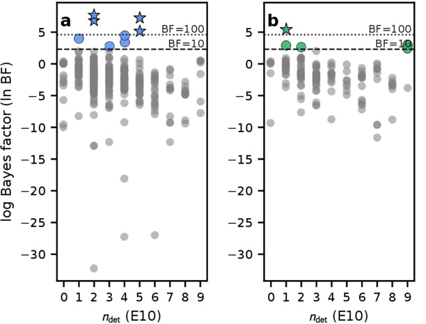
Evidence for a model including technologically processed material relative to a purely natural model, as a function of the number of elements detected in the white dwarf. ndet = 0 indicates that only upper limits were obtained on elemental abundances. Higher Bayes factors indicate stronger evidence. The left-hand plot is based on abundances measured from the white dwarfs’ photospheres, while the right-hand plot uses abundances adjusted for diffusion within the white dwarf. Click to enlarge. [Adapted from Huang et al. 2026]

No Strong Evidence, but a Path Forward

Ultimately, Huang’s team found that strong statistical support for the existence of technological processes was uncommon, though there were certain measurements in their sample of white dwarfs that were difficult to reconcile with a solely natural model.

Perhaps unsurprisingly, the team also found that the quality of the chemical abundance measurements affected the constraining power of the observation; some white dwarfs had upper limits for just a few elements, while others had definitive detections of many elements. They found that the most discerning observations recorded iron, magnesium, chromium, and titanium, plus either nickel, silicon, or sodium.

While this work didn’t dredge up firm evidence for technological activity, it provides a jumping-off point for future searches. The handful of white dwarfs in this sample that were fit poorly by a purely natural model could be compared against other technosignature models or targeted with high-resolution spectroscopy. Future measurements of iron and magnesium in polluted white dwarfs may be useful as a preliminary screening tool, helping to pick out intriguing targets for follow-up observations.

Citation

“A Calibrated Bayesian Search for Potential Chemical Technosignatures in Polluted White Dwarfs,” Bo-Lun Huang et al 2026 ApJ 1006 9. doi:10.3847/1538-4357/ae742c

The post Seeking Technosignatures in Polluted White Dwarfs appeared first on AAS Nova.

Can Arid Planets Keep Their Cool?

14 July 2026 at 17:00

side-by-side images of Venus's surface today and an imagining of what its surface might have looked like in the past

Editor’s Note: Astrobites is a graduate-student-run organization that digests astrophysical literature for undergraduate students. As part of the partnership between the AAS and astrobites, we occasionally repost astrobites content here at AAS Nova. We hope you enjoy this post from astrobites; the original can be viewed at astrobites.org.

Title: Carbon Cycle Imbalances on Arid Terrestrial Planets with Implications for Venus
Authors: Haskelle T. White-Gianella and Joshua Krissansen-Totton
Authors’ Institution: University of Washington
Status: Published in PSJ

The Carbon-Cycle Thermostat

When discussing the habitability of planets, we usually focus on the habitable zone, the region around a star where a planet can host a temperature suitable for supporting liquid water on its surface. Yet, being in the right place doesn’t necessarily guarantee that a planet will be habitable.

A planet also needs the right atmospheric composition to sustain the necessary temperatures for hosting liquid water. A key mechanism found on Earth for maintaining this composition is the geologic carbon cycle, which acts as a built-in climate control system. This cycle begins with volcanic eruptions releasing carbon dioxide (CO2), which then dissolves in rainwater and forms a weak acid that weathers rocks on continents. The weathering products wash into oceans, where they form carbonate rocks, locking carbon away. Eventually, plate tectonics recycles some of that carbon back to volcanoes. The weathering process works faster when the planet is warmer, thus regulating the amount of CO2 and stabilizing the climate over long periods of time (but it should be noted that it can take up to a few hundred thousand years to rebalance this slow carbon cycle through the weathering process).

An important caveat is that the weathering process requires sufficient liquid water on the planet’s surface, so what happens in the case for planets with shallower oceans? Low-mass M dwarfs, the most common type of star found in the galaxy, are expected to host less-massive disks and therefore lower water inventories for forming planets. If more “dry” planets are indeed a more likely outcome of planet formation, we’d want to know how their arid conditions influence their long-term evolution and habitability.

Creating Carbon-Tracking Models

The authors built a model that tracks how water and CO2 move between a planet’s interior, oceans, and atmosphere over 4.5 billion years. The model notably includes the following:

  • A sophisticated weathering model that accounts for how runoff can limit rock weathering, improving upon previous models that only included a temperature dependence on weathering
  • Wind-driven evaporation limits that influence the amount of water evaporation in addition to sunlight-driven evaporation
  • Multiple deep water cycle parameterizations that explore how water moves between the interior and the surface

The model tests for four initial surface water inventories (0.1%, 1%, 10%, and 100% of Earth’s oceans) and then simulates how the surface water, atmosphere, and climate evolve over time.

A Critical Water Threshold

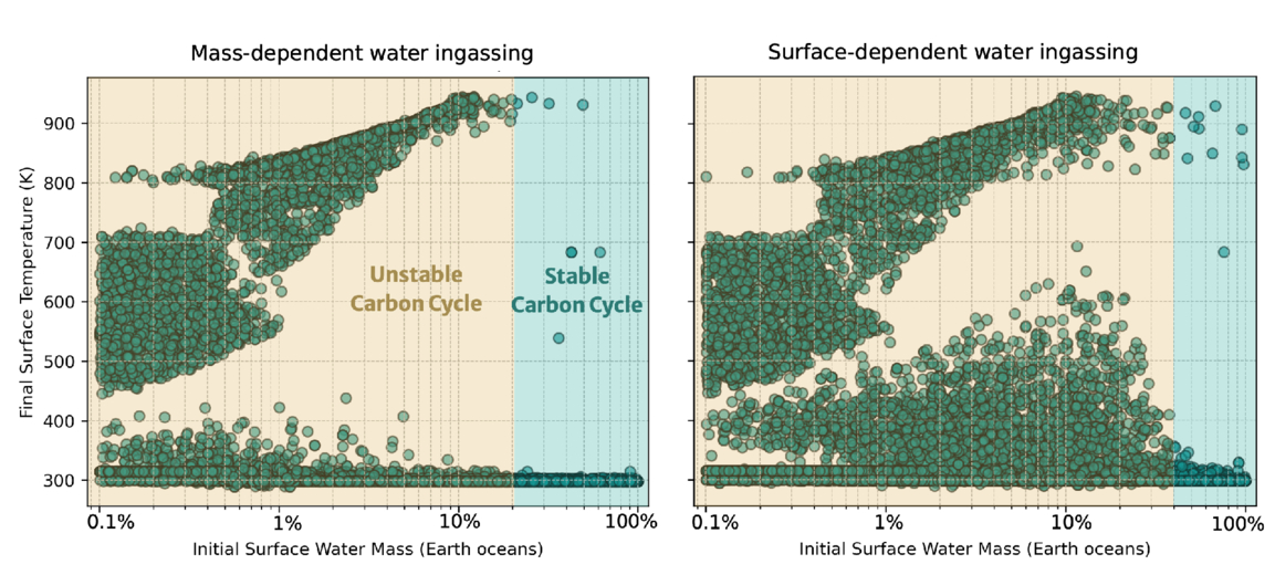
The models reveal that planets require at least 20–50% of Earth’s ocean mass to maintain a balanced carbon cycle. Below this threshold, the carbon cycle becomes unbalanced, leading to devastating consequences for habitability (Figure 1).

two plots of final surface temperature as a function of initial surface water mass

Figure 1: Final surface temperature after simulating 4.5 billion years of evolution as a function of initial water inventory for Earth-like planets. Each dot represents a model run with different assumptions (total carbon inventory, temperature dependence of weathering, soil age, etc.). The yellow region shows where most simulations result in uninhabitable surface temperatures from an unbalanced carbon cycle, and the cyan region shows where most simulations result in habitable surface temperatures and a balanced carbon cycle. The left and right plots show the results for two different parameterizations of the deep water cycle implemented in the model. [White-Gianella & Krissansen-Totton 2026]

For the more arid planets, models reveal a concerning runaway process. Limited surface water reduces precipitation and slows rock weathering. Weathering cannot keep up with volcanic CO2 release, causing CO2 buildup and warming of the atmosphere. The cycle repeats, driving runaway warming until all water evaporates.

Important Implications (Within and Outside Our Solar System)

Looking within the solar system, the results offer an explanation for how a potentially habitable Venus could have transitioned into its current inhospitable state. If Venus had formed with an initial water inventory below this critical threshold of 20–50% of Earth’s ocean mass, then its carbon cycle would have become unbalanced, creating the CO2 inferno seen on Venus today.

In future exoplanet studies, telescopes like the Habitable Worlds Observatory might detect ocean glint (specular reflection from liquid water) or measure land fraction from light curves. Finding a planet in the habitable zone but with limited ocean coverage would likely be bad news, as the planet could be quietly losing its grip on habitability. Astronomers may want to be more careful when looking at seemingly promising planets within their habitable zones.

Original astrobite edited by Natalie Price.

About the author, Jared Bull:

I am a 2nd-year PhD student at Johns Hopkins University. I study brown-dwarf variability and am interested in using time-series observations to uncover dynamic processes within their atmospheres. In my free time I like to read, cook, and do astrophotography.

The post Can Arid Planets Keep Their Cool? appeared first on AAS Nova.

When the Spacecraft Align: Rescuing Saturated Images of Solar Flares

13 July 2026 at 17:00

close-up image of the Sun showing a solar flare

Many observations of solar flares suffer from saturation and blooming, causing crucial information to be lost. Researchers recently validated a technique for retrieving information from saturated flare images, unlocking a treasure trove of powerful solar flares for examination.

Solutions for Saturation

Since 2010, the Atmospheric Imaging Assembly (AIA) on the Solar Dynamics Observatory (SDO) has been capturing nearly continuous extreme-ultraviolet images of the Sun’s disk, revealing our star’s dramatic high-energy behavior. Though SDO/AIA’s observations have transformed our understanding of the Sun’s activity, they have limitations: powerful solar flares can saturate the detector, spilling charge into nearby pixels.

This saturation and overflow compromises our ability to study the most energetic solar flares — but the “lost” information may actually be recoverable. When light from an intense flare enters SDO’s instruments, not all of it pools in the saturated region of the detector: some of the light is diffracted by the optics, and by mathematically inverting this pattern of diffracted light, researchers can attempt to extract the encoded information about the saturated region. Researchers have used this technique for more than a decade, but options for validating the results were limited until now.

Solar Orbiter Lends a Hand

Launched almost 10 years to the day after SDO, the Solar Orbiter spacecraft provides an excellent opportunity to test inversion techniques for recovering information from saturated solar images. Solar Orbiter’s Extreme Ultraviolet Imager snaps brief photos of the Sun at a rapid cadence, and its images remain unsaturated even when faced with energetic solar flares.

positions of Solar Dynamics Observatory and Solar Orbiter during a solar flare on 19 March 2024

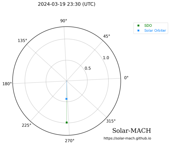
Positions of SDO (green) and Solar Orbiter (blue) during a solar flare on 19 March 2024. Click to enlarge. [Guastavino et al. 2026]

As described in a recent research article by Sabrina Guastavino (University of Genoa; Italian National Institute for Astrophysics) and collaborators, the ideal setup for testing the inversion technique arose on 19 March 2024, when SDO and Solar Orbiter both viewed a solar flare while separated by just 1 degree in longitude.

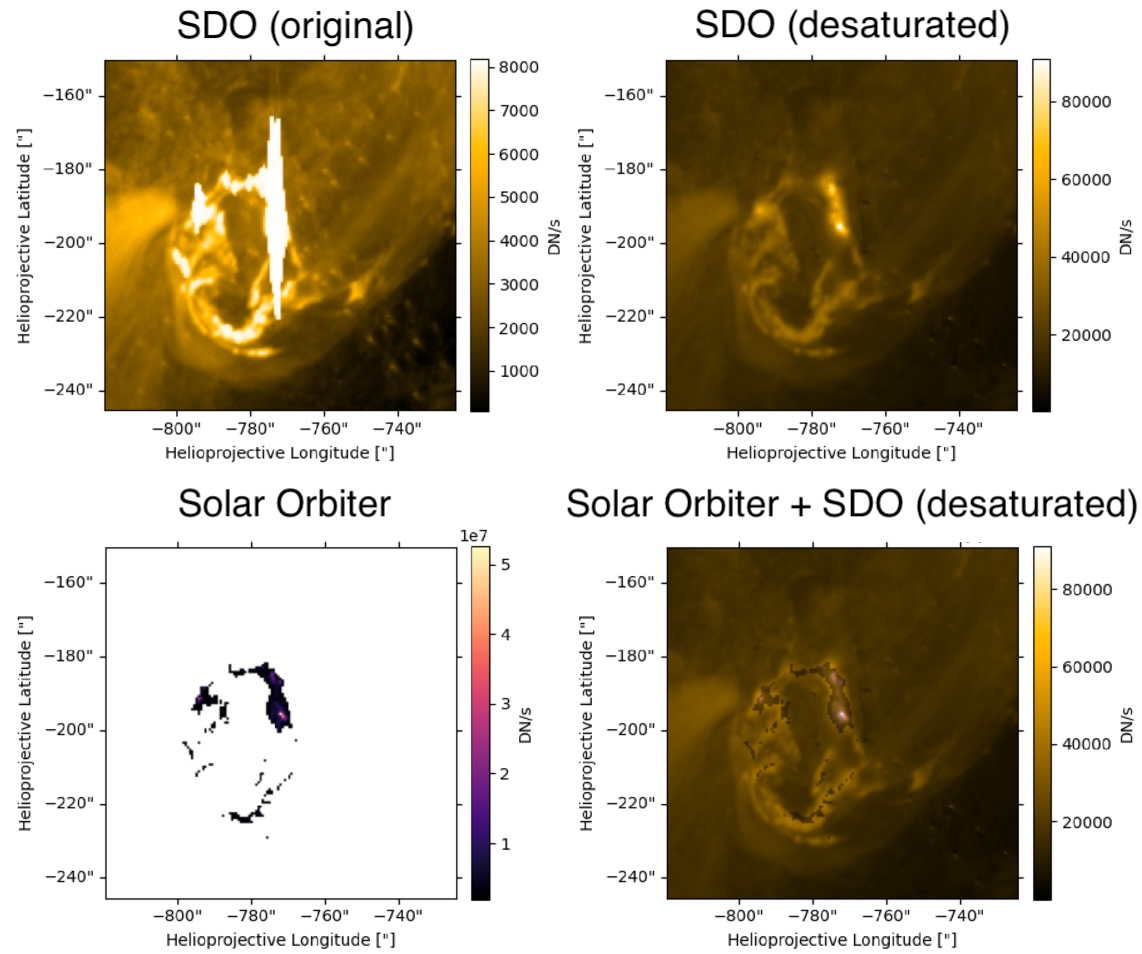
Guastavino’s team aligned and reprojected the data, accounting for the slightly different viewing angles of the two spacecraft, then applied an algorithm called Adaptive SE-DESAT to reconstruct the flux within the saturated portion of the SDO image. The team compared the desaturated SDO images to the unsaturated Solar Orbiter images over the course of the flare, finding the same flare morphology and similar time evolution between the two data sets.

sample results of the desaturation process

Example of unprocessed SDO data (top left), desaturated SDO data (top right), Solar Orbiter data (bottom left), and a combination of the two data sources (bottom right). Note that the Solar Orbiter observations have been clipped so that only the highest flare intensities were recorded. Click to enlarge. [Adapted from Guastavino et al. 2026]

A Treasure Trove of Desaturated Data

Overall, these results demonstrate the effectiveness of the inversion technique, though Guastavino and coauthors noted that improvements could be made during the impulsive phase of the flare, when the emission is increasing. The team identified several reasons why the results may not match during this phase, including rapid evolution of the flare during individual exposures.

Despite these areas that require further attention, the validation of this technique unlocks 16 years of solar flare observations from SDO. This especially enhances our sample of powerful solar flares, increasing the available records of the most energetic solar flares by orders of magnitude.

Citation

“Validation of an Extreme-Ultraviolet Desaturation Technique for the Atmospheric Imaging Assembly on Board the Solar Dynamics Observatory Using Observations from the Extreme Ultraviolet Imager on Board Solar Orbiter,” Sabrina Guastavino et al 2026 ApJL 1005 L50. doi:10.3847/2041-8213/ae7d2e

The post When the Spacecraft Align: Rescuing Saturated Images of Solar Flares appeared first on AAS Nova.

Putting the Landing Site Before the Lander

10 July 2026 at 17:00

An oblique-angle photograph of a deep crater half in shadow.

NASA is once again sending scientific missions to the Moon. But under the new commercial framework for getting there, researchers need to invent a new method for how to pick where to land.

A New Process for Picking Sites

NASA’s Commercial Lunar Payload Services program is a bold innovation in organizing robotic missions to the Moon. Under this model, rather than keeping the mission process entirely in-house, the agency selects the scientific mission they want to support then simply buys a ride to the lunar surface from a commercial vendor. But, how do you pick a landing site before you know exactly how you’re getting there?

A photograph from orbit of two volcanic mounds on the moon.

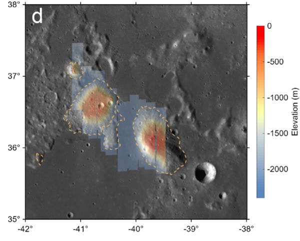
The Gruithuisen domes region, the broad area the Lunar-VISE team searched for potential landing sites. Click to enlarge. [Adapted from Williams et al. 2026]

The Lunar Vulkan Imaging and Spectroscopy Explorer (Lunar-VISE) mission, set to launch in mid-2028, was one of the first programs to go through this new landing site selection process. After being officially selected in 2022, the team had just nine months to nail down exactly where their mission should touch down. A recent article led by Jean-Pierre Williams (University of California, Los Angeles) detailed exactly how the team accomplished this task and presented some lessons they learned along the way.

No Parking Lots on the Moon

Picking a landing site is no small task: for context, selecting the landing sites for each of the most recent Mars rovers took five years and multiple community workshops. The Lunar-VISE team therefore took a streamlined and logic-driven approach. They started by explicitly laying out their science objectives: Lunar-VISE’s purpose is to investigate some strangely silicate-rich volcanic formations called the Gruithuisen domes, so they had to land either on or near those. They also had to have access to boulders that were excavated from deep within the domes during a crater formation event, so they had to pick a spot with boulders relatively nearby.

In addition to objectives, they also laid out a slew of constraints. Although they needed boulders nearby, they couldn’t have too many boulders, or any particularly large boulders, since those could pose hazards for landing. There also couldn’t be any steep slopes in the field. Most of the area had to maintain a line of sight with a supporting orbiter for communications, so they couldn’t set down near any ridges. Also, they had to consider how the terrain would cast shadows as the lunar day progressed, since they didn’t want their mission cut short by freezing temperatures and a lack of solar power. As the team quipped, “many interesting, high-science value locations on the Moon may not be in proverbial ‘parking lots.'”

A low-angle photo of a crater and plain on the moon, with arrows and annotations to the landing ellipse, boulders, and the edge of the dome.

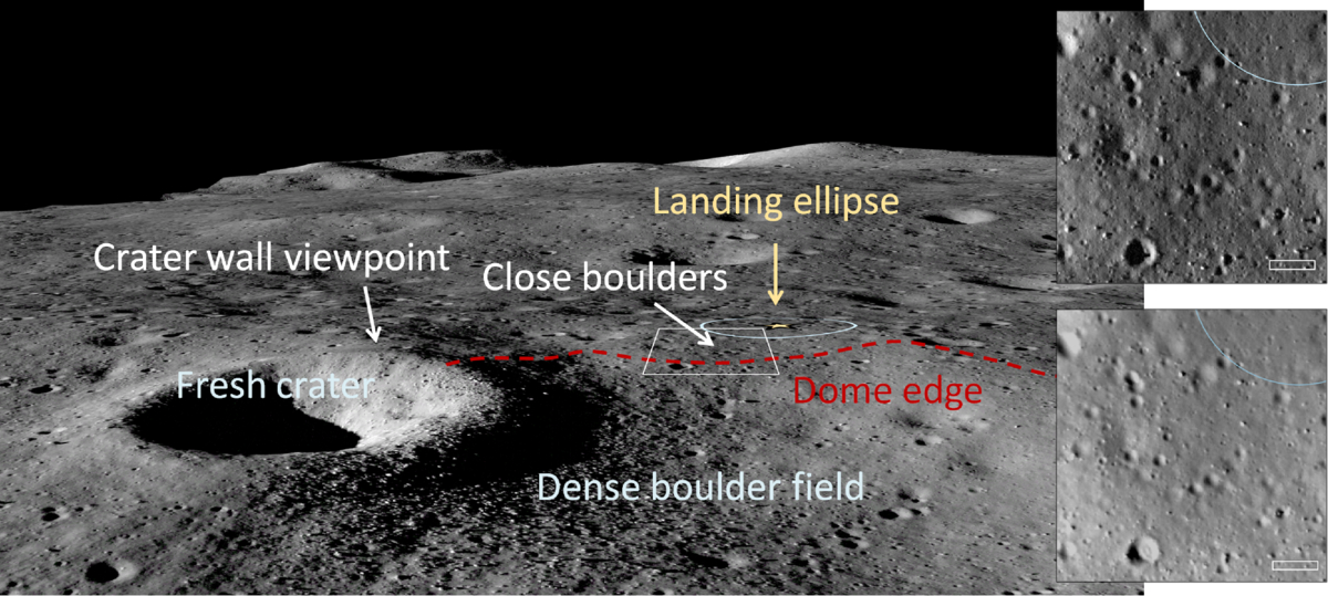
An image from the Lunar Reconnaissance Orbiter overlaid onto a terrain model of the final landing site. Click to enlarge. [Williams et al. 2026]

By combing through archival data and working with the team that operates the Lunar Reconnaissance Orbiter Camera, a key asset for making detailed maps of the Moon, the researchers found the perfect spot: alongside a 190-meter-diameter crater named Mareta. This feature is named after Mareta West, one of the first female planetary geologists at the United States Geological Survey and the scientist who selected the landing site for Apollo 11’s historic touchdown.

In addition to presenting their landing site, the researchers offered a handful of lessons to others who may someday be in the fortunate and thrilling position of needing to pick a landing spot on the Moon. For one, they urged teams to coordinate with the Lunar Reconnaissance Orbiter specialists as early as possible, since processing the imaging data for lander-quality maps is a specialized and intensive task. For another, they recommended that all of the software tools used be made publicly available so that future missions don’t need to duplicate their work.

As this article laid out, the Commercial Lunar Payload Services program and Lunar-VISE take us one step closer to making missions to the Moon routine — but we’re still figuring out exactly how to do that.

Citation

“Lunar-VISE Landing Site Selection and Characterization at Mons Gruithuisen Gamma,” Jean-Pierre Williams et al 2026 Planet. Sci. J. 7 161. doi:10.3847/PSJ/ae7d2c

The post Putting the Landing Site Before the Lander appeared first on AAS Nova.

Gaia Data Show That the Initial Mass Function Is Not Universal

8 July 2026 at 22:48

star-forming cloud OMC-2

Do all star-forming regions birth stars with the same distribution of masses? Theory suggests that they do not, but researchers often assume they do for simplicity. Now, ultra-precise observations from Gaia have demonstrated that the initial mass function varies across star clusters in the Milky Way.

A Universal Initial Mass Function?

JWST image of galaxies in the iconic Hubble Ultra Deep Field

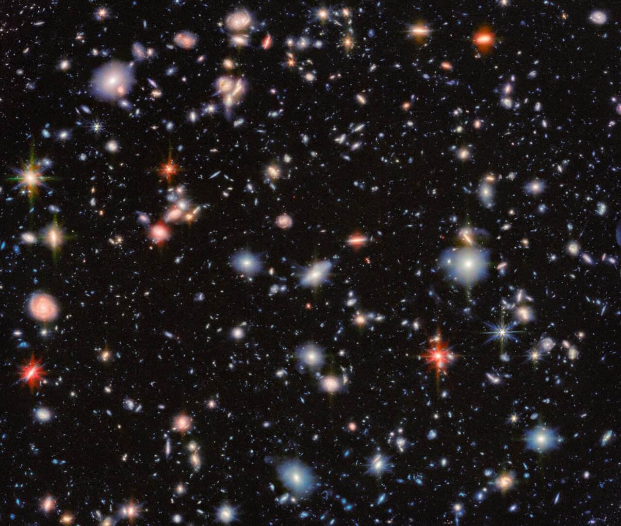
The light from distant galaxies is dominated by high-mass stars, requiring the use of the IMF to estimate the stellar mass of a galaxy. [ESA/Webb, NASA & CSA, G. Östlin, P. G. Perez-Gonzalez, J. Melinder, the JADES Collaboration, the MIDIS collaboration, M. Zamani (ESA/Webb); CC BY 4.0]

When a molecular cloud fragments, collapses, and births a star cluster, how many stars form, and what are their masses? The answer to that question is what astronomers term the initial mass function, or IMF: the distribution of masses of stars born in a cluster.

The IMF is important in many areas of astronomy, and it’s relied on especially heavily in studies of distant galaxies. The light from these galaxies is dominated by high-mass stars, with the emission from lower-mass stars lost in the glare, so astronomers must use the IMF to reconstruct the stellar populations of these far-off locales.

Though theory suggests that the IMF should vary with factors like temperature and metallicity, demonstrating these variations has been difficult, even within our own galaxy. Because of this, researchers often adopt a universal IMF drawn from observations of star clusters in the Milky Way. But is the IMF truly universal?

The More the Slope Changes, the More the Break Mass Stays the Same

Determining whether the IMF is universal is more complicated than simply comparing the stars in one cluster to those in another. That’s because what astronomers measure in present-day star clusters is not the initial mass function, but a version of the IMF that has been skewed by millions to billions of years of evolution; over time, high-mass stars die and low-mass stars get ejected, warping the shape of the mass function.

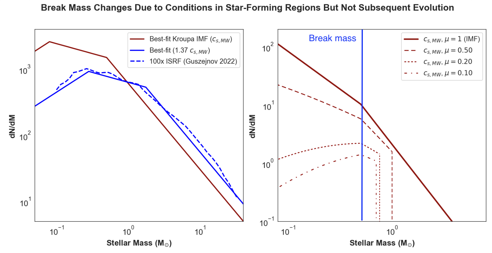
Plots of the stellar mass function

Left: Different break masses arise for different properties (here, the sound speed) of a given star-forming cloud. Right: Evolution of the mass function over time for a single star cluster. Over time, high-mass stars die and low-mass stars are ejected from the cluster, resulting in a decrease in the remaining mass fraction, μ, from 1 to 0.1. The slopes change, but the break mass does not. Click to enlarge. [Adapted from Steinhardt et al. 2026]

However, as demonstrated in a recent research article led by Charles L. Steinhardt (University of Missouri), certain aspects of the IMF may remain unchanged as clusters evolve. When the mass function of a star cluster is described using a broken power law (commonly called a “Kroupa-like” IMF in reference to work by Pavel Kroupa), the slopes of the power-law segments are affected by stellar evolution and dynamical interactions. Crucially, these effects appear not to alter the break mass — the mass at which the IMF transitions from one slope to another. Therefore, differences in the break mass from cluster to cluster reflect differences in the underlying IMF rather than the stellar and dynamical evolution of the clusters.

Insights from Gaia

Thanks to the Gaia spacecraft, which made precise observations of more than 2 billion stars in the Milky Way and beyond, it’s now possible to measure and compare the break masses of individual star clusters. Out of an initial catalog of 7,167 Milky Way clusters observed with Gaia, Steinhardt’s team selected just 110 that were of high enough quality and contained a sufficient number of stars to measure cluster break masses accurately.

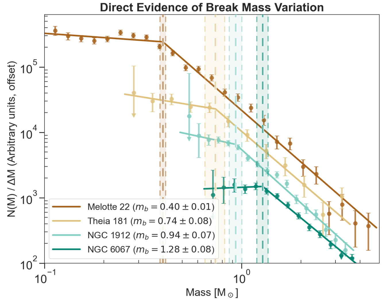
Plot of stellar mass function for four Milky Way clusters

Observed mass functions of four Milky Way star clusters. The break masses are clearly different, showing that the IMF must vary from cluster to cluster. Click to enlarge. [Steinhardt et al. 2026]

The team found that the break mass differs considerably between the clusters in their sample, showing that the IMF is not universal. The observed variety of break masses appears to be linked to the age of the cluster, but instead of reflecting the impact of stellar and dynamical evolution — which have no effect on the break mass — these differences reflect the properties of the clouds in which the clusters were born. This implies that the properties of star-forming clouds in the Milky Way have, on average, changed over cosmic time. Thus, a star cluster that formed billions of years ago would have had a different IMF than one forming today.

This finding has implications for studies of high-redshift galaxies, where the properties of star-forming clouds are markedly different from those in the Milky Way. Going forward, Steinhardt and coauthors recommend developing a flexible parameterization of the IMF to capture how this critical function behaves in environments vastly different from our own.

Citation

“Direct Evidence for Stellar Initial Mass Function Variation in the Milky Way,” Charles L. Steinhardt et al 2026 ApJL 1005 L40. doi:10.3847/2041-8213/ae7444

The post Gaia Data Show That the Initial Mass Function Is Not Universal appeared first on AAS Nova.

Distant Galaxies: Dead or in Disguise?

7 July 2026 at 17:00

distant starburst galaxies

Editor’s Note: Astrobites is a graduate-student-run organization that digests astrophysical literature for undergraduate students. As part of the partnership between the AAS and astrobites, we occasionally repost astrobites content here at AAS Nova. We hope you enjoy this post from astrobites; the original can be viewed at astrobites.org.

Title: MAGAZ3NE: Confirming Dust Deficiency and Quiescent Nature of Ultramassive Galaxies at 3 < z < 4 with ALMA Observations
Authors: Wenjun Chang et al.
First Author’s Institution: University of California, Riverside
Status: Published in ApJ

Distant galaxies offer a unique window into how stars, gas, and dust evolve over cosmic time. Tracing this evolution requires understanding not only how galaxies form, but also how and when they stop forming stars, a process known as quenching. Understanding how, when, and why galaxies quench is a fundamental question in astrophysics, and one that requires observations of star-forming, quenching, and fully quenched galaxies alike. Unfortunately, one complication is that identifying truly quenched galaxies is challenging: galaxies that appear “dead” may instead be actively forming stars, hidden behind a thick veil of dust.

In today’s article, the authors use observations from the Atacama Large Millimetre/submillimetre Array (ALMA) to investigate five ultramassive galaxies at redshifts, z, between 3 and 4, and ask a deceptively simple question: are these massive red galaxies genuinely quenched, or are they secretly forming stars behind the scenes?

Meet the Suspects: Ultramassive Galaxies at the Edge of Cosmic Noon

The five galaxies in this study are drawn from the Massive Ancient Galaxies at z > 3 NEar-infrared (MAGAZ3NE) survey, which targets some of the most massive galaxies known at early cosmic times. All five have stellar masses exceeding 100 billion solar masses and have been confirmed at z > 3. At these redshifts, we are observing the galaxies as they were when the universe was less than 2 billion years old. This is just before an epoch known as cosmic noon, when star formation across the universe reached its peak.

These galaxies also benefit from extensive multiwavelength observations from a range of observatories, including the ground-based Visible and Infrared Survey Telescope for Astronomy and the Spitzer Space Telescope. By combining imaging across wavelengths from the ultraviolet to the near-infrared, astronomers can measure the “colours” of galaxies and use these colours to infer the galaxies’ star-forming activity.

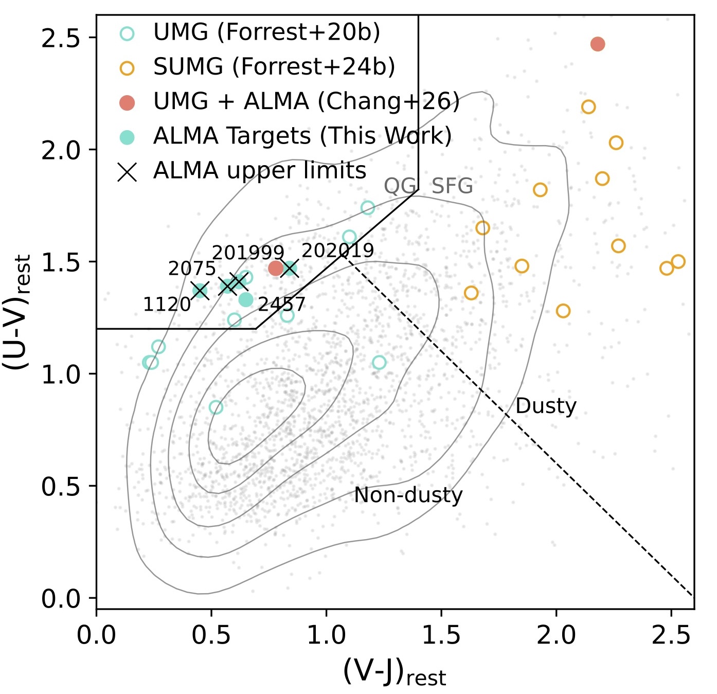
Galaxies that have quenched their star formation are dominated by older stellar populations, which makes them appear red (hence why they are often referred to as “red and dead” galaxies). However, dust can redden galaxies in a similar way by absorbing blue light and re-emitting it at longer wavelengths — meaning that a dusty, star-forming galaxy can easily masquerade as a quenched one. To uncover any hidden star formation, the authors turn to ALMA to search for far-infrared dust emission. The sample of galaxies investigated with ALMA is shown in Figure 1.

UVJ color–color diagram

Figure 1: UVJ colour–colour diagram, which uses galaxy colours in the ultraviolet (U), visible (V), and near-infrared (J) to identify quenched galaxies. The five ultramassive galaxies (UMGs) studied here (filled cyan circles) lie firmly in the quenched region (QG), consistent with a lack of ongoing star formation. Crosses indicate galaxies undetected in ALMA dust emission, while other massive galaxies at similar redshifts are shown in grey for comparison. [Chang et al. 2026]

ALMA on the Scene

ALMA observes light at sub-millimetre wavelengths, which at these redshifts traces emission from star-forming regions that are obscured by dust. Of the five ultramassive galaxies in this sample, only one is detected with ALMA. Even when the remaining four galaxies are stacked together, no dust emission is recovered, indicating that if any dust is present, it must be extremely faint.

To better quantify what these ALMA non-detections imply, the authors perform spectral energy distribution fitting (see a recent overview bite on spectral energy distribution fitting) using the Code Investigating GALaxy Emission, or CIGALE, a code that enforces energy balance between absorbed starlight and dust emission to estimate physical properties such as a galaxy’s star formation rate and dust content. With the ALMA constraints included, all five galaxies are found to lie more than 10 times below the star-forming main sequence. Even the single ALMA-detected galaxy remains formally quenched, showing only weak residual star formation.

In other words, these galaxies really are dead (or at least extremely dormant).

Extremely Dust-Poor Galaxies

The spectral energy distribution fitting also allows the authors to measure how much dust these galaxies contain relative to their stellar mass. This ratio provides a simple but powerful way to assess how much interstellar material remains in a galaxy — and therefore how much fuel is left for future star formation.

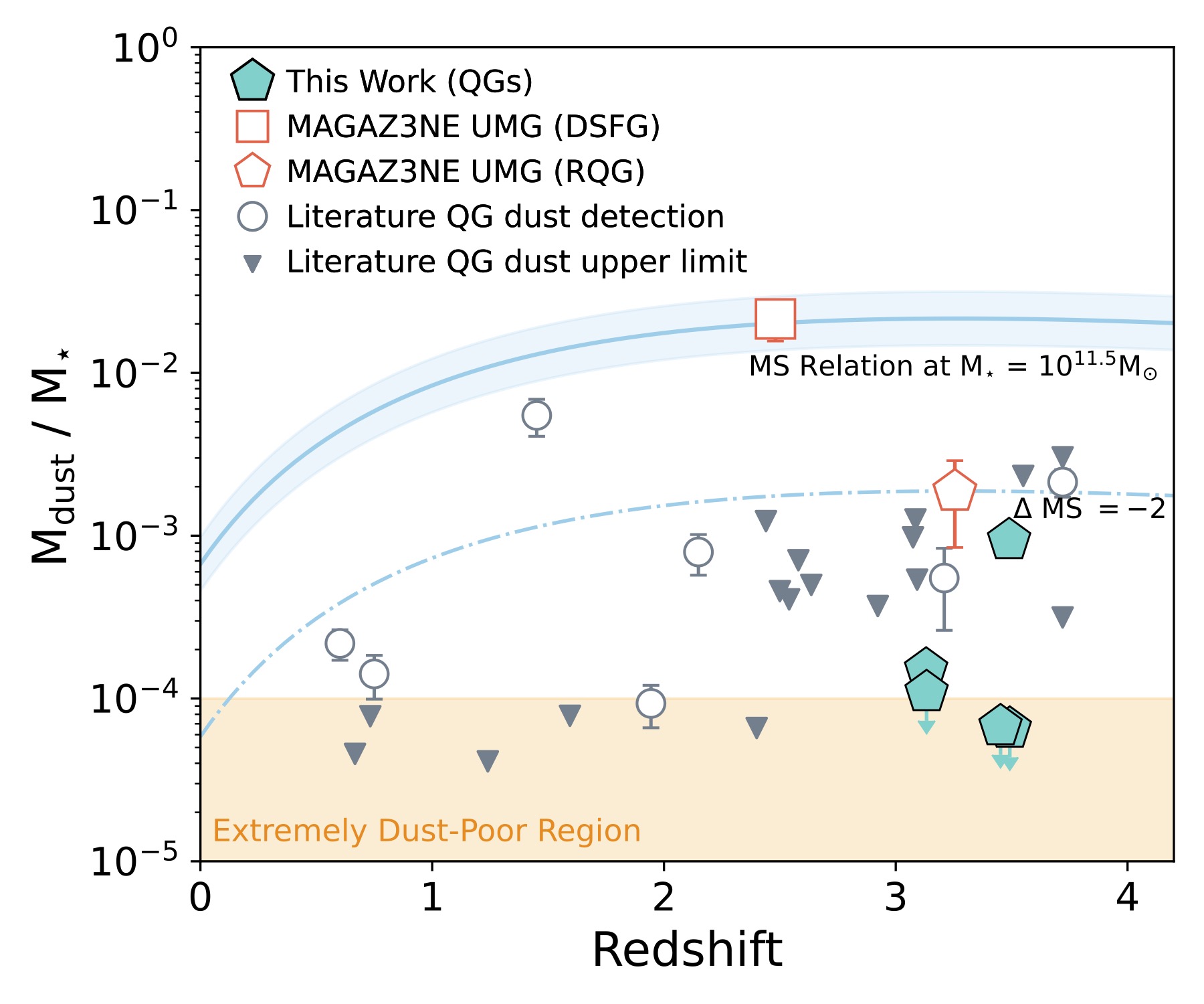
Three of the five ultramassive galaxies have ratios of Mdust/Mstar < 10-4 (Figure 2), placing them among the most dust-poor quenched galaxies confirmed at z > 3. The lone galaxy detected by ALMA contains slightly more dust, with Mdust/Mstar = 10-3, but even this is far below what would be expected for an actively star-forming galaxy. For comparison, typical star-forming galaxies at similar stellar masses host more than 100 times more dust.

Plot of dust-to-stellar mass ratio versus redshift

Figure 2: The ratio of dust mass to stellar mass versus redshift for massive quenched galaxies (QGs). This quantity measures how dust rich a galaxy is compared to its stellar mass. The ultramassive galaxies in this study (cyan pentagons) fall well below the dust content expected for star-forming galaxies (solid blue line), highlighting their extreme dust deficiency. [Adapted from Chang et al. 2026]

These results raise important questions about how galaxies can become ultramassive, quenched, and nearly dust-free within the first two billion years of cosmic history.

For now, ALMA has delivered a clear answer to the question of “dead or in disguise?”: at least some candidate ultramassive galaxies in the early universe really are quenched, and they are strikingly dust poor. By ruling out the dusty impostor scenario, this study shows that deep ALMA observations can cleanly distinguish genuinely quenched galaxies from dusty star-forming ones, even at the highest stellar masses and earliest cosmic times. How these galaxies lost their dust remains an open question, but one thing is clear: by the time cosmic noon arrived, some galaxies had already finished forming stars and quietly faded into dormancy.

Original astrobite edited by Viviana Cáceres.

About the author, Lucie Rowland:

I’m a fourth (and final!) year PhD student at Leiden Observatory in the Netherlands, studying massive, star forming galaxies in the early universe with ALMA and JWST. It’s a really exciting time to be interested in astronomy, so I hope to make groundbreaking new research more accessible!

The post Distant Galaxies: Dead or in Disguise? appeared first on AAS Nova.

Featured Image: A Mass Mystery in the Bullet Cluster

6 July 2026 at 17:00

Bullet Cluster with mass countours

The Bullet Cluster is best known for being considered a “smoking gun” for the existence of dark matter, but even a famous galaxy cluster like this one has its secrets. For more than two decades, different measurements of the merging clusters’ dynamical mass ratio have yielded vastly different results. In a recent research article, Boseong Young Cho (Yonsei University) and collaborators used data from JWST and the Dark Energy Camera to revisit the Bullet Cluster and measure its mass ratio using new data. The image above shows a near-infrared view of the Bullet Cluster from JWST, with an overlay of mass contours derived from gravitational-lensing measurements. The team’s analysis assigned a mass of 1.5 quadrillion solar masses for the main cluster (on the left side of the image above), and a mass of 150 trillion solar masses for the subcluster. This suggests a mass ratio of roughly 10, which matches the value supported by hydrodynamical simulations and cements the event as a minor merger. The team also identified three distinct cluster halos (two in the main cluster and one in the subcluster), providing an important constraint on the cluster configuration for future modeling. To learn more about this investigation of the Bullet Cluster, be sure to check out the full research article linked below!

Citation

“Joint JWST–DECam Lensing Reveals that the Bullet Cluster Is a Minor Merger,” Boseong Young Cho et al 2026 ApJ 1005 28. doi:10.3847/1538-4357/ae6a90

The post Featured Image: A Mass Mystery in the Bullet Cluster appeared first on AAS Nova.

A New Catalog of Stellar Rotation Periods for Over a Million Stars

1 July 2026 at 18:22

TESS in space

Stellar rotation is a crucial aspect of not only stellar evolution but also exoplanet science, and a recent study has built the largest catalog of stellar rotation periods to date.

Stellar Opportunities with TESS

Since its launch in 2018, the Transiting Exoplanet Survey Satellite (TESS) has scoured the sky, searching for the signature recurring dip in starlight caused by planetary companions. While the primary goal of TESS is to discover exoplanets, the satellite’s mapping of the entire sky has created a rich database of high-quality photometry for millions of stars. These observations offer ample opportunity for scientists to study stellar properties and behavior across the Milky Way.

In particular, stellar rotation is a key property that traces a star’s age, magnetic activity, and internal structure. For exoplanet science, stellar rotation is both a help and a hindrance: it allows us to study how exoplanets may evolve over time with their host stars, but stellar activity can mimic or drown out planet signals, making them harder to detect. A few studies have investigated stellar rotation periods with TESS, looking at specific star clusters and known planet hosts. To date, however, no existing study has produced a larger catalog of TESS rotation periods — a product that would provide a wealth of information for both exoplanet and stellar evolution science.

Creating a Catalog

TESS All-Sky Rotation Survey

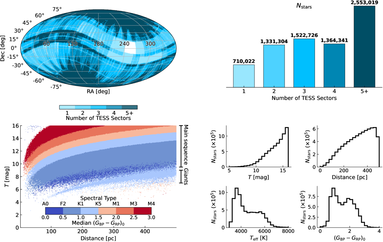
Target sample summary showing the TESS sky coverage (top left), histogram of number of TESS observations per star (top right), TESS magnitude as a function of distance to the star (bottom left), and histograms of magnitude, distance, temperature, and color across the sample (bottom right). Click to enlarge. [Boyle et al 2026]

Seeking to build a flux- and distance-limited catalog of TESS rotation periods, Andrew W. Boyle (The University of North Carolina at Chapel Hill) and collaborators used TESS full-frame images to survey the local neighborhood for stellar variability. To measure reliable stellar rotation periods for as large and diverse a sample as possible, the authors made selection cuts in brightness, distance, and data availability to build a target sample of 7,481,412 stars. They generated light curves for each observation of each star and searched them for periodicity, or repeated variation in brightness.

Not all brightness variations present in a star’s light curve are due to stellar variability — instrumental systematics and artifacts from the spacecraft’s orbital period can produce periodic variability. To combat this, the authors created a classification algorithm to select sources whose periodicity is most likely due to true stellar variability rather than instrumental or observational effects. Pairing this classification with some additional validation criteria, the authors built the TESS All-Sky Rotation Survey (TARS), a catalog of periods for 1,046,317 stars within about 1,600 light-years of our Sun.

Map of fast rotators in TARS sample

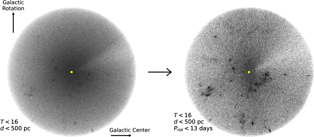
Map of all TARS stars within about 1,600 light-years of the Sun (left) and only the fast-rotating stars in the survey, highlighting clustered populations (right). Click to enlarge. [Boyle et al 2026]

Implications of TARS

Looking more finely at the TARS catalog, the authors provided additional quality cuts to remove other potential sources of stellar variability like binary companions or pulsations. The authors estimated that roughly 93% of their measured periods are due to stellar rotation, which expands the number of stars with known rotation periods by a factor of 2.3 within about 325 light-years and by a factor of 4.0 within about 1,600 light-years. As the largest homogeneous catalog of stellar rotation periods to date, TARS lays the groundwork for studies of stellar evolution, exoplanet discovery and evolution, and even Milky Way structure. For example, the authors found that when mapping the fast-rotating, typically younger stars in TARS, the location of young stellar associations in the local neighborhood became significantly clearer. This underscores the importance of this catalog for a range of science goals, and future work will only improve upon the data provided by TARS.

Citation

“The TESS All-Sky Rotation Survey: Periods for 1,046,317 Stars within 500 pc,” Andrew W. Boyle et al 2026 ApJS 284 75. doi:10.3847/1538-4365/ae6657

The post A New Catalog of Stellar Rotation Periods for Over a Million Stars appeared first on AAS Nova.

Two More Thoughts on Little Red Dots

1 July 2026 at 03:54

little red dots seen with JWST

One of the biggest discoveries from JWST’s tenure is a population of compact reddish objects nicknamed “little red dots.” Numerous theories have been proposed to explain the small sizes, high luminosities, and characteristic “V”-shaped spectra of these objects, and today we’ll examine two recent research articles that have explored the identity of the universe’s most mysterious inhabitants.

Red Dot, Blue Dot

You can tell a lot about a person by looking at their friends — and the same might be true for little red dots. A team led by Josephine Baggen (Yale University) examined a sample of 83 little red dots imaged with JWST. They found that 43% of the little red dots in this sample had a little blue companion: an ultraviolet-bright object within a projected separation of 1,630–16,300 light-years. The brightest little red dots were even more likely to have a blue companion; 80% of the brightest objects in the sample were paired up.

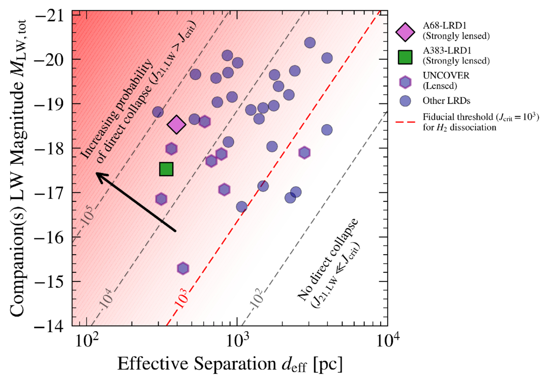
Baggen’s team set out to test the hypothesis that these red–blue pairs are fundamentally linked rather than coincidental. Under this hypothesis, the ultraviolet-bright blue companions were assembled first. The ultraviolet radiation from these objects suppressed the cooling of molecular hydrogen in pristine gas clouds in the early universe, causing the gas to skip the usual star-forming process and instead form a massive compact object such as a black hole star, supermassive star, or quasi-star — which we see as a little red dot.

plot of Lyman-Werner radiation versus projected separation

The companion’s mean flux density from 91.2 to 111 nm versus projected separation between the blue companion and the little red dot. The red dashed line shows the estimated values necessary for gas clouds to collapse. Click to enlarge. [Baggen et al. 2026]

Baggen and coauthors investigated whether the ultraviolet radiation from the blue companions is strong enough to have triggered this transformation. The team used spectral energy distribution modeling to determine the luminosities of the blue companions from 91.2 to 111 nanometers. This analysis showed that the radiation from the blue companions is equal to or greater than the threshold necessary to encourage the direct collapse of a gas cloud into a massive compact object.

If little red dots form thanks to their little blue companions, that would imply that every little red dot has or had such a companion. Though little blue companions weren’t so universal in the sample used in this work, the team noted that their analysis techniques, combined with observational limitations and other factors, likely yielded a smaller number of blue companions than are actually present. Further simulations exploring the collapse of pristine gas clouds into massive compact objects and high-resolution spectroscopic observations of little red dots can illuminate the potential link between these objects.

globular cluster NGC 1851

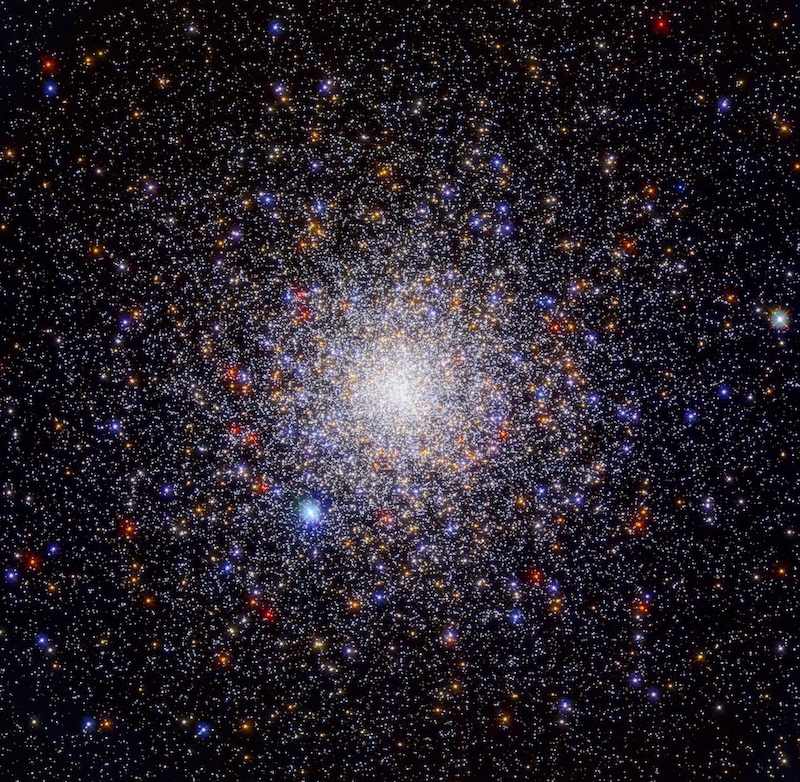
The densely packed globular cluster NGC 1851, as seen by the Hubble Space Telescope. [NASA, ESA, and G. Piotto (Università degli Studi di Padova); Processing: Gladys Kober (NASA/Catholic University of America)]

Little Red Dots as Young Globular Clusters

John Chisholm (The University of Texas at Austin) and collaborators hypothesized that little red dots represent a brief phase in the formation of globular clusters. In this hypothesis, the rest-frame ultraviolet emission of little red dots comes from the hot young stars of the newborn cluster, while the rest-frame optical emission comes from a single supermassive star at the cluster’s heart. Thus, in this framework, the little red dot phase lasts only as long as the fleeting lifespan of the supermassive star.

Chisholm’s team first showed that the spectrum of a young globular cluster with a supermassive star at its center is similar to the observed spectrum of a little red dot. But showing that the emission properties of globular clusters in formation and little red dots are similar is not enough — it’s also necessary to investigate whether the numbers and masses of these objects line up.

mass functions of little red dots and globular clusters

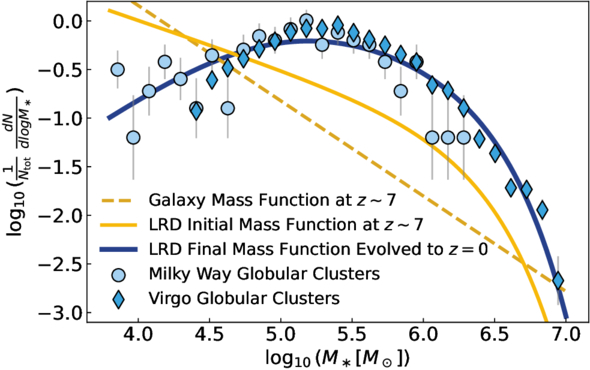
Comparison of the mass functions of little red dots evolved forward to the present day (blue line) and globular clusters in the Milky Way and Virgo (blue symbols). The results for both populations have been normalized to emphasize the shape of the distributions. Click to enlarge. [Chisholm et al. 2026]

To do this, the team propagated the observed mass function of little red dots at a redshift of z = 7 forward in time to z = 0. This process accounted for the rapid evolution of the supermassive star into a black hole, as well as the evolution of and feedback from the massive stars in the cluster. Comparing the resulting mass function to the population of present-day globular clusters, the team found that the mass functions had very similar shapes, and the number densities of little red dots and globular clusters in the present day are estimated to be of the same order of magnitude: 0.1–0.3 Mpc-3 and 0.8 Mpc-3, respectively.

In addition to describing how the properties of globular clusters in formation match those of little red dots, Chisholm’s team outlined some testable predictions for this scenario, including formation timescales and chemical abundance patterns. If this hypothesis withstands further scrutiny, little red dots may provide a valuable look at the early years of some of our universe’s oldest star clusters.

Citation

“Connecting the Dots: UV-Bright Companions of Little Red Dots as Lyman–Werner Sources Enabling Direct-Collapse Black Hole Formation,” Josephine F. W. Baggen et al 2026 ApJL 1002 L4. doi:10.3847/2041-8213/ae58a5

“Little Red Dots as Globular Clusters in Formation,” John Chisholm et al 2026 ApJL 1004 L4. doi:10.3847/2041-8213/ae6dae

The post Two More Thoughts on Little Red Dots appeared first on AAS Nova.

A Wandering Supermassive Black Hole Eating a Star

29 June 2026 at 17:00

disk of hot gas swirling around a black hole

Editor’s Note: Astrobites is a graduate-student-run organization that digests astrophysical literature for undergraduate students. As part of the partnership between the AAS and astrobites, we occasionally repost astrobites content here at AAS Nova. We hope you enjoy this post from astrobites; the original can be viewed at astrobites.org.

Title: The Wandering Supermassive Black Hole Powering the Off-Nuclear Tidal Disruption Event AT2024tvd
Authors: M. Guolo et al.
First Author’s Institution: Johns Hopkins University
Status: Published in ApJL

A Star Gets Eaten in the Wrong Neighborhood

We find supermassive black holes at the centers of most large galaxies. They end up there because of how galaxies form: as matter collapses and merges over time, material sinks to the gravitational center, and the black hole settles in.

So, what happens when we catch a star being ripped apart by a supermassive black hole that is not at the center of its galaxy?

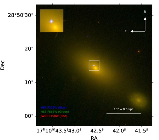
That is exactly the puzzle posed by AT2024tvd, a tidal disruption event (TDE) spotted roughly 2,600 light-years from the center of a massive galaxy located 600 million light-years away from us (see Figure 1).

AT2024tvd from Hubble and JWST

Figure 1: A color image of AT2024tvd from the Hubble Space Telescope and JWST. The yellow dot inside the square marks the galaxy’s center, while the TDE is the white dot, which is visibly offset to the upper left, about 2,600 light-years away. [Adapted from Guolo et al. 2026]

We see TDEs when a black hole tears apart a star that gets too close to it. It happens because the black hole’s gravity pulls harder on the near side of the star than the far side, stretching the star until it comes apart. The stellar debris then forms a hot accretion disk, a ring of material swirling around the black hole that spirals inward and releases a burst of electromagnetic energy across many wavelengths — from visible light to X-rays. These events are valuable to astronomers because they briefly light up black holes that would otherwise be invisible, giving us a rare window to measure their properties. Since supermassive black holes live at galactic centers, that is also where we expect TDEs to happen, which makes a TDE found away from a galactic center rare and puzzling. The galactic center is often called the nucleus of a galaxy, so astronomers refer to these displaced events as “off-nuclear” TDEs. AT2024tvd is only the third known off-nuclear TDE, and this research article makes a strong case that it is the most remarkable one yet.

Measuring Mass Using Light

To figure out the mass of the black hole responsible for AT2024tvd, the authors needed to get creative. You cannot weigh a black hole directly, so astronomers have to work backward from what they can see. The key idea is that a black hole’s mass controls how its accretion disk behaves. A more massive black hole produces a larger, cooler disk, while a less massive one produces a smaller, hotter disk. By measuring how bright the disk is at different wavelengths and how hot it gets, you can figure out how massive the black hole must be.

The authors did this by modeling the light the event produced across many wavelengths. They combined data from several telescopes: the Zwicky Transient Facility, the Neil Gehrels Swift Observatory, Pan-STARRS, and two rounds of high-quality X-ray data from XMM-Newton. TDE light curves go through different phases. The early flare in visible and ultraviolet light is bright but complicated, and the physical processes behind it are not fully understood. But after a few hundred days, TDEs settle into a quieter “plateau phase,” where the ultraviolet and visible light come directly from the accretion disk. At this stage, the emission follows well-understood physics, and astronomers can model it reliably.

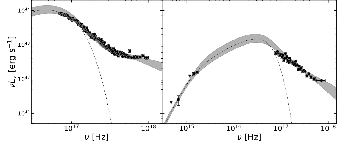
The authors used a model called kerrSED, which describes the spectral energy distribution (SED) of a spinning black hole’s accretion disk (kerr). It accounts for the disk’s temperature, its physical size, the black hole’s spin (how fast it rotates), and the angle at which we are viewing the system. It also accounts for a process called Comptonization, where hot electrons near the black hole boost lower-energy photons (particles of light) up to X-ray energies. By fitting this model to the observed light at multiple wavelengths simultaneously, the authors could pin down the disk properties and extract the black hole mass. The result was a clean fit: the disk model alone could explain all the observed light during the plateau phase, with nothing significant left over (see Figure 2).

brightness evolution of AT2024tvd

Figure 2: The brightness of AT2024tvd measured across a wide range of wavelengths, after correcting for absorption and the galaxy’s motion. The symbols show individual measurements from different telescopes, while the shaded contours represent the best-fit disk model and its uncertainty. Left: The early X-ray data, which is well explained by emission from the hot inner accretion disk. Right: The later data covering both visible/ultraviolet light and X-rays, all consistently explained by the same disk model. [Adapted from Guolo et al. 2026]

Not an Intermediate, but a Supermassive Black Hole

From their fit, the authors found a black hole mass of about one million solar masses. Black holes above about 100,000 solar masses are considered supermassive, while those below that threshold but above about 100 solar masses are called intermediate-mass black holes. So, this puts AT2024tvd in the supermassive category. This matters because the two previously known off-nuclear TDEs, called 3XMM J2150-05 and EP240222a, were both powered by intermediate-mass black holes. Those black holes were found inside small, dense collections of stars called ultra-compact dwarf galaxies that were orbiting larger host galaxies.

AT2024tvd is different. When the authors looked at deep images of the location where the TDE happened, they found no star cluster or small galaxy there. Whatever group of stars once surrounded this black hole has been almost entirely pulled apart by the gravity of the much larger parent galaxy. The ratio of the black hole’s mass to the mass of any remaining stars around it is extreme: greater than 3%, which is far above what we normally see. This is the signature of a “wandering” supermassive black hole, one that was brought in during a past galaxy merger and has been slowly sinking toward the center of its new host ever since, losing its surrounding stars along the way.

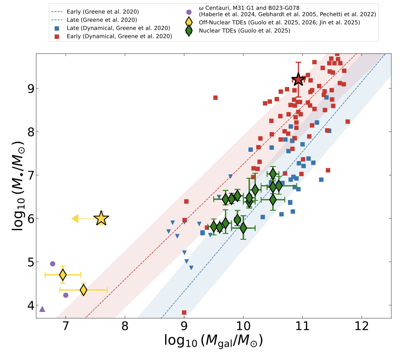
The authors compared AT2024tvd to other TDEs using established relationships between accretion disk properties and black hole mass (Figure 3). In terms of its disk temperature, luminosity, and inferred mass, AT2024tvd behaves like a typical nuclear TDE powered by a supermassive black hole. However, when placed on the black hole mass versus host stellar mass relation, it stands out as a strong outlier. The black hole mass is far too large for the small amount of surrounding stellar mass detected at its location.

plot of black hole mass versus host galaxy mass

Figure 3: AT2024tvd (yellow star) plotted on the relationship between black hole mass and host galaxy stellar mass. Red squares show nearby galaxies with dynamically measured black hole masses plotted against galaxy bulge stellar mass, while blue squares show the relation using total galaxy stellar mass. Purple points and green diamonds represent nuclear TDE host galaxies with black hole masses inferred from different TDE modeling techniques. Yellow diamonds mark the two previously known off-nuclear TDEs. AT2024tvd stands out as a clear outlier, with a very high black hole mass compared to the upper limit on any surrounding stellar mass. [Guolo et al. 2026]

The Big Picture

This discovery matters for several reasons. It shows that off-nuclear TDEs are not limited to intermediate-mass black holes sitting in small satellite galaxies. Some are powered by fully supermassive black holes that have been displaced from their original galactic centers. It also shows that TDE modeling, when done carefully during the plateau phase of the light curve (when the emission is dominated by well-understood accretion disk physics), can provide reliable black hole masses on its own, without assuming any relationship between the black hole and its host galaxy. This is particularly important for wandering black holes, where those relationships do not apply.

Looking ahead, upcoming surveys like Vera C. Rubin Observatory’s Legacy Survey of Space and Time are expected to find many more off-nuclear TDEs. Combined with X-ray follow-up from telescopes like XMM-Newton, these events could become our main tool for mapping out the population of displaced black holes in the nearby universe. One disrupted star at a time, we are starting to find black holes that theory told us should exist but that had, until now, stayed hidden.

Original astrobite edited by Kelsie Taylor and Veronika Dornan.

About the author, Serat Saad:

Serat is a first-year PhD student in astronomy at The Ohio State University. His research is on stellar and galactic dynamics, where he uses observational data to understand gravity. He also has interests in active galactic nuclei and tidal disruption events.

The post A Wandering Supermassive Black Hole Eating a Star appeared first on AAS Nova.

Detached but Not Alone

26 June 2026 at 17:00

A rendering of a Jupiter-like planet floating in front of a galaxy.

Microlensing surveys have discovered plenty of regular exoplanets, but more surprisingly, they’ve also turned up many solo Neptunes with no star nearby. New research suggests that first impressions might be deceiving, however, and that at least some of these planets might not be so alone: they just have a complicated family history.

An Abundance of Exo-Neptunes

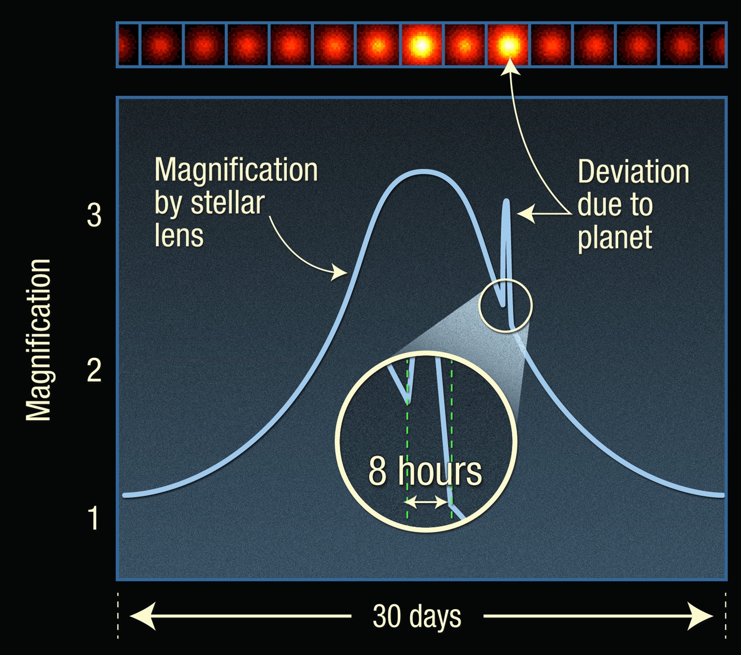
There are simply too many Neptune-like exoplanets in our galaxy. Or at least that’s the current feeling astronomers get from gravitational microlensing surveys, which look for exoplanets during short-lived magnification events caused by chance alignments between stars. These surveys have now found about a dozen so-called “free-floating” planets, and while this doesn’t sound like that many, running the numbers reveals that this tiny sample implies that there are about two free-floating Neptune-size planets for every star in the galaxy.

A schematic graph of a large pulse and a smaller narrower pulse superimposed on top.

An illustration of how exoplanets are found via microlensing. The broad first bump is caused by the host star magnifying the light from a background star; the narrow second bump is caused by the planet acting as a lens as well. “Free-floating” planets create only one bump. [Adapted from NASA, ESA, and A. Feild (STScI)]

The idea that there are more free-ranging Neptunes than stars is unsettling, and astronomers aren’t yet sure how this many planets ended up so isolated. It’s possible that these objects simply formed disconnected from any planetary system, but it’s unclear how something so small could collapse from the interstellar clouds that usually produce stellar-mass objects. It’s also possible that the planets formed around stars in the usual way, only to be later kicked out by some violent dynamical process — but this would either require too much time or too many giant planets capable of ejecting the lower-mass ones.

However, new research by Sam Hadden (Canadian Institute for Theoretical Astrophysics) and Yanqin Wu (University of Toronto) presents an alternative idea: what if at least some of these free-floating planets aren’t fully on their own, but instead remain estranged but weakly bound to their parent stars?

Simulated Scattering

Two celestial objects need to align nearly perfectly in order to create a microlensing pulse that we can detect. For an exoplanet orbiting a star, we should observe two of these pulses: one when the host star drifts in and out of alignment with a background star, and one when the nearby bound planet does the same. In the case of a free-floating planet, there’s only one pulse, and we therefore assume that there is no host star. Hadden and Wu noticed that since the alignment has to be so precise for microlensing to occur, it’s possible that a seemingly free-floating planet is simply widely separated from its host star, and the star managed to dodge the magnification effect. In other words, these planets might not be free floating at all, just on wide and eccentric orbits.

A two-panel plot showing how the semimajor axis and inclination of 5 planets evolve over time.

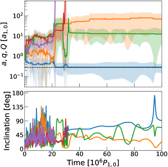
The orbital evolution of a five-planet system that undergoes planet–planet scattering. Each line represents one planet; note that in the end two are ejected, two end up on wide detached orbits, and the fifth ends up on a tightly bound inner orbit. Click to enlarge. [Hadden & Yu 2026]

The researchers decided to test whether it’s possible to create these kinds of orbits via a known dynamical process called planet–planet scattering. As the name implies, during this process, planets that begin on orderly orbits around their parent star undergo a dramatic rearrangement as they jostle each other around through gravitational interactions. The researchers created two types of simulations: one with a collection of equal-mass planets, and another in which one planet dominates over a brood of smaller ones. After setting up the systems, they let the “dynamical havoc” proceed for a few hundred million years, then surveyed the aftermath.

They found that both types of simulations readily created the “detached” objects needed to mimic free-floating planets. In fact, the most common outcome was for two or three planets to be bullied into far-out orbits by a planet that then plunges onto a tight inner orbit extremely close to the star.

Though the authors caution that this process likely doesn’t explain all of the free-floating planets observed to date, this is an exciting model that would dramatically lower our estimates of the number of Neptunes roaming alone between the stars.

Citation

“Free Floating or Merely Detached?,” Sam Hadden and Yanqin Wu 2026 ApJ 1000 70. doi:10.3847/1538-4357/ae6508

The post Detached but Not Alone appeared first on AAS Nova.

New Spectral Signs of Buckyballs Discovered in Planetary Nebula

24 June 2026 at 17:00

illustration of buckyballs in a planetary nebula

Fullerenes — a class of molecules composed entirely of interconnected carbon atoms — are the largest molecules definitively detected in space. Researchers using JWST to study a planetary nebula have found new spectral features from a fullerene composed of 60 carbon atoms, offering another way to study how these molecules form and survive in space.

Full of Fullerenes

planetary nebula Tc 1

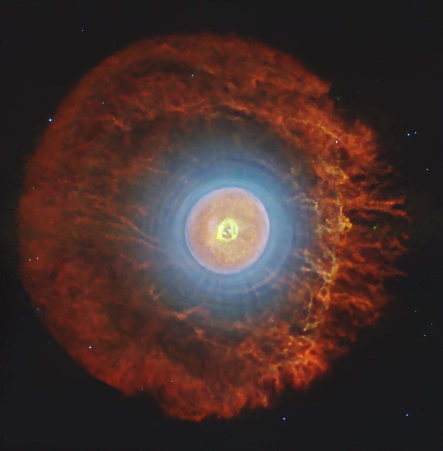
Planetary nebula Tc 1 as seen by JWST. [NASA / ESA / CSA / Western University, J. Cami]

The planetary nebula Tc 1 holds special significance in the field of astrochemistry. More than a decade ago, researchers using the Spitzer Space Telescope studied this wispy nebula illuminated by the core of a dead star. These observations led to the first confident identification of molecules called fullerenes in space. Fullerenes are large molecules constructed from interconnected rings of carbon atoms, forming hollow spheres, rugby-ball shapes, and long tubes. Spheroidal fullerenes, especially C60, are commonly referred to as buckyballs.

Since that discovery, Tc 1 has been a hot spot for studies of buckyballs. However, researchers are still puzzling over how these large molecules form and survive in harsh space environments.

closeup of planetary nebula Tc 1

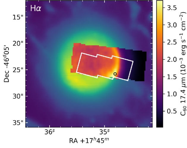
A closeup of the center of Tc 1, showing the region observed with JWST’s Mid-Infrared Instrument (black-to-yellow color scale) and Near-Infrared Spectrograph (white outline). The background color scale shows the nebula’s H-alpha emission as seen by the Very Large Telescope. [Adapted from Giese et al. 2026]

From Spitzer to JWST

Morgan Giese (The University of Western Ontario) and collaborators recently reported on the results of a JWST observing program that aimed to understand how fullerenes respond to changes in their environment. The team mapped the distribution of C60 molecules at varying distances from the powerful ionizing radiation of Tc 1’s central star.

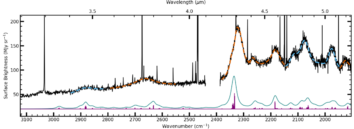
The team successfully spotted the emission features from the fullerene C60 seen in earlier observations, but they also turned up something unexpected: a handful of prominent emission features from 3.5 to 5.2 microns that had not been reported previously.

Feature Presentation

What’s the source of these emission features? The distribution of the emission provides a strong clue: known spectral features from fullerenes C60 and C70 are concentrated in a narrow, bright ring around the center of the nebula, with diffuse emission suffusing the rest of the nebula — and the newfound spectral features follow the same distribution.

JWST spectrum of Tc 1

JWST spectrum of Tc 1 (black line) extracted from the area indicated by a black circle in the previous image. The orange and blue dashed lines show fits to the newfound emission bands, and the results of the anharmonic calculations are shown as the teal line below the JWST spectrum. Click to enlarge. [Giese et al. 2026]

This evidence hints that C60 or C70 is the source of these new features, but Giese’s team took the investigation a step further. Using anharmonic quantum chemical calculations, they computed the spectrum of C60‘s combination bands, which arise when multiple vibrational modes are excited at the same time. This is the first time this type of spectrum has been calculated for C60, and the authors found good agreement between their computed spectrum and the JWST spectrum, providing further evidence that C60 is the source of these bands.

Giese and coauthors found that 17% of the energy emitted by the C60 molecules in Tc 1 is released in these  combination bands, suggesting that these features must be taken into account when modeling the cooling of C60 molecules. The discovery of new fullerene spectral features also has implications for future studies of these molecules: since these features appear in a wavelength range where features from other complex molecules like polycyclic aromatic hydrocarbons are weak, these newly identified bands provide a promising way to spot and study fullerenes across space environments.

Citation

“Detection of C60 Combination Bands in the Near-IR Spectrum of Tc 1,” Morgan M. Giese et al 2026 ApJL 1004 L32. doi:10.3847/2041-8213/ae76d5

The post New Spectral Signs of Buckyballs Discovered in Planetary Nebula appeared first on AAS Nova.

❌