❌

Normal view

Noble Gases Along for the Ride

24 July 2026 at 17:00

A rendering of an orange and grey planet against a dark background.

What can some neon trapped in a chunk of rock tell us about Earth’s formation and the protosolar nebula? Quite a lot, as detailed in a recent study in The Planetary Science Journal.

Noble Mysteries

By analyzing rocks pulled from mid-ocean ridges, geologists have concluded that there are tiny amounts of noble gases in the deep interior of Earth. That’s a strange statement upon reflection: how did these gases, which are famously apathetic to essentially all other elements, end up embedded within rocks thousands of kilometers underground? Since their passivity rules out the potential of a chemical reaction that formed them in place, they must have been in the mantle since the very beginning of Earth’s history.
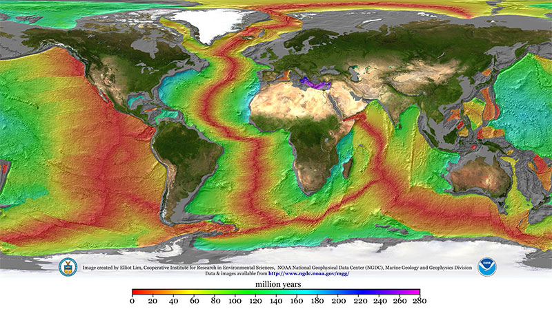
A map of Earth with the continents shown normally but the sea colored according to age.

A map illustrating the age of the seafloor. Mid-ocean ridges stand out clearly in red. By sampling material from these ridges, planetary scientists can infer the composition of Earth’s deep interior. Click to enlarge. [Mr. Elliot Lim, CIRES and NOAA/NCEI]

There are a few scenarios for how this could have happened. Though it’s possible that these inert species were delivered to the early Earth encapsulated within primitive meteorites or in solids contaminated by ions from the solar wind, at least some fraction of these elements likely came directly from the gaseous nebula that surrounded the earliest protoplanets.

That last option is especially exciting to present-day planetary scientists interested in constraining Earth’s formation history because it requires some very specific conditions. Since light noble gases like neon don’t dissolve well in seawater, they must have dissolved into a magma ocean — meaning the nebula was still around when Earth was large enough to have a molten surface. That already restricts us to a very specific time in the solar system’s history, but it doesn’t say much about the specific size of the proto-Earth other than “big,” and it doesn’t say much about the state of the nebula other than “it existed.” Recently, Vincent Savignac and Eve Lee (University of California, San Diego; McGill University) successfully refined these constraints to pin down information about both the early Earth and the nebula that surrounded it.

Infant Earths

Savignac and Lee began by growing a grid of infant Earths on their computers via models of gas accretion and atmosphere–magma interactions. Each simulation started with a different proto-Earth mass and nebular density, and each one yielded a different amount of neon in Earth’s deep interior. Excitingly, only a small handful of the scenarios tested ended up with values similar to those observed.
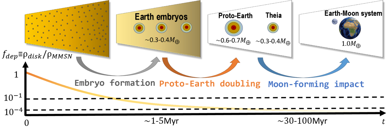
A cartoon of small cores surrounded by gaseous envelopes eventually merging into the Earth.

A schematic of Earth’s formation via embryo formation (when the noble gases enter the mantle) followed by mergers. Click to enlarge. [Savignac & Lee 2026]

On the mass axis, the team found a narrow range of acceptable conditions. If a proto-Earth was less than about 20% of Earth’s present-day mass, it couldn’t accrete much gas. This let it cool rapidly, freezing the magma ocean and shutting down neon dissolution before too much could be trapped inside. On the other hand, if a proto-Earth was more than about 40% of Earth’s present-day mass, it would accrete too much gas, stay molten for too long, and be left with too much neon. On the density axis, the researchers found that when the nebula accreted on to the proto-Earth, it must have been fairly depleted compared to its initial density. This implies that the whole process happened at the end of the nebula’s life, just before it was completely blown away by the proto-Sun.

Savignac and Lee demonstrated that these constraints are robust against the later stages of Earth’s evolution. In its later years, Earth either suffered or benefited from a giant impact, depending on your feelings about the Moon, but the researchers showed that this event doesn’t pose a problem for their models. Overall, this study builds a delightful link between rocks from our deep oceans and the particulars of Earth’s formation, demonstrating the unique power of planetary science to tie together different scientific fields.

Citation

“Constructing the Earth’s Formation History Using Deep Mantle Noble Gas Reservoirs,” Vincent Savignac and Eve J. Lee 2026 Planet Sci. J. 7 135. doi:10.3847/PSJ/ae64f7

The post Noble Gases Along for the Ride appeared first on AAS Nova.
Putting the Landing Site Before the Lander

10 July 2026 at 17:00

An oblique-angle photograph of a deep crater half in shadow.

NASA is once again sending scientific missions to the Moon. But under the new commercial framework for getting there, researchers need to invent a new method for how to pick where to land.

A New Process for Picking Sites

NASA’s Commercial Lunar Payload Services program is a bold innovation in organizing robotic missions to the Moon. Under this model, rather than keeping the mission process entirely in-house, the agency selects the scientific mission they want to support then simply buys a ride to the lunar surface from a commercial vendor. But, how do you pick a landing site before you know exactly how you’re getting there?

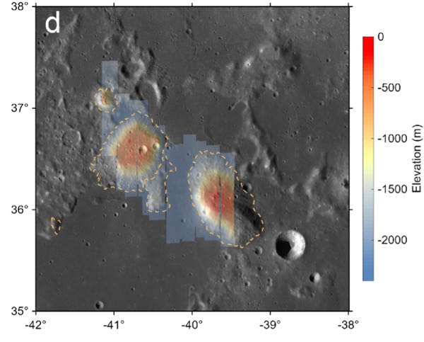
A photograph from orbit of two volcanic mounds on the moon.

The Gruithuisen domes region, the broad area the Lunar-VISE team searched for potential landing sites. Click to enlarge. [Adapted from Williams et al. 2026]

The Lunar Vulkan Imaging and Spectroscopy Explorer (Lunar-VISE) mission, set to launch in mid-2028, was one of the first programs to go through this new landing site selection process. After being officially selected in 2022, the team had just nine months to nail down exactly where their mission should touch down. A recent article led by Jean-Pierre Williams (University of California, Los Angeles) detailed exactly how the team accomplished this task and presented some lessons they learned along the way.

No Parking Lots on the Moon

Picking a landing site is no small task: for context, selecting the landing sites for each of the most recent Mars rovers took five years and multiple community workshops. The Lunar-VISE team therefore took a streamlined and logic-driven approach. They started by explicitly laying out their science objectives: Lunar-VISE’s purpose is to investigate some strangely silicate-rich volcanic formations called the Gruithuisen domes, so they had to land either on or near those. They also had to have access to boulders that were excavated from deep within the domes during a crater formation event, so they had to pick a spot with boulders relatively nearby.

In addition to objectives, they also laid out a slew of constraints. Although they needed boulders nearby, they couldn’t have too many boulders, or any particularly large boulders, since those could pose hazards for landing. There also couldn’t be any steep slopes in the field. Most of the area had to maintain a line of sight with a supporting orbiter for communications, so they couldn’t set down near any ridges. Also, they had to consider how the terrain would cast shadows as the lunar day progressed, since they didn’t want their mission cut short by freezing temperatures and a lack of solar power. As the team quipped, “many interesting, high-science value locations on the Moon may not be in proverbial ‘parking lots.'”

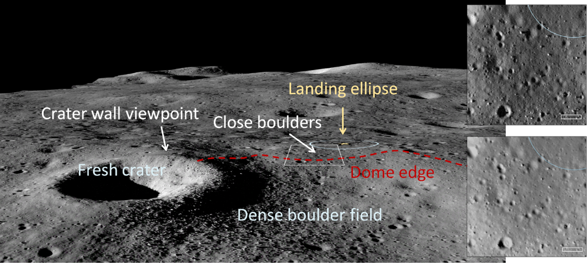
A low-angle photo of a crater and plain on the moon, with arrows and annotations to the landing ellipse, boulders, and the edge of the dome.

An image from the Lunar Reconnaissance Orbiter overlaid onto a terrain model of the final landing site. Click to enlarge. [Williams et al. 2026]

By combing through archival data and working with the team that operates the Lunar Reconnaissance Orbiter Camera, a key asset for making detailed maps of the Moon, the researchers found the perfect spot: alongside a 190-meter-diameter crater named Mareta. This feature is named after Mareta West, one of the first female planetary geologists at the United States Geological Survey and the scientist who selected the landing site for Apollo 11’s historic touchdown.

In addition to presenting their landing site, the researchers offered a handful of lessons to others who may someday be in the fortunate and thrilling position of needing to pick a landing spot on the Moon. For one, they urged teams to coordinate with the Lunar Reconnaissance Orbiter specialists as early as possible, since processing the imaging data for lander-quality maps is a specialized and intensive task. For another, they recommended that all of the software tools used be made publicly available so that future missions don’t need to duplicate their work.

As this article laid out, the Commercial Lunar Payload Services program and Lunar-VISE take us one step closer to making missions to the Moon routine — but we’re still figuring out exactly how to do that.

Citation

“Lunar-VISE Landing Site Selection and Characterization at Mons Gruithuisen Gamma,” Jean-Pierre Williams et al 2026 Planet. Sci. J. 7 161. doi:10.3847/PSJ/ae7d2c

The post Putting the Landing Site Before the Lander appeared first on AAS Nova.

Detached but Not Alone

26 June 2026 at 17:00

A rendering of a Jupiter-like planet floating in front of a galaxy.

Microlensing surveys have discovered plenty of regular exoplanets, but more surprisingly, they’ve also turned up many solo Neptunes with no star nearby. New research suggests that first impressions might be deceiving, however, and that at least some of these planets might not be so alone: they just have a complicated family history.

An Abundance of Exo-Neptunes

There are simply too many Neptune-like exoplanets in our galaxy. Or at least that’s the current feeling astronomers get from gravitational microlensing surveys, which look for exoplanets during short-lived magnification events caused by chance alignments between stars. These surveys have now found about a dozen so-called “free-floating” planets, and while this doesn’t sound like that many, running the numbers reveals that this tiny sample implies that there are about two free-floating Neptune-size planets for every star in the galaxy.

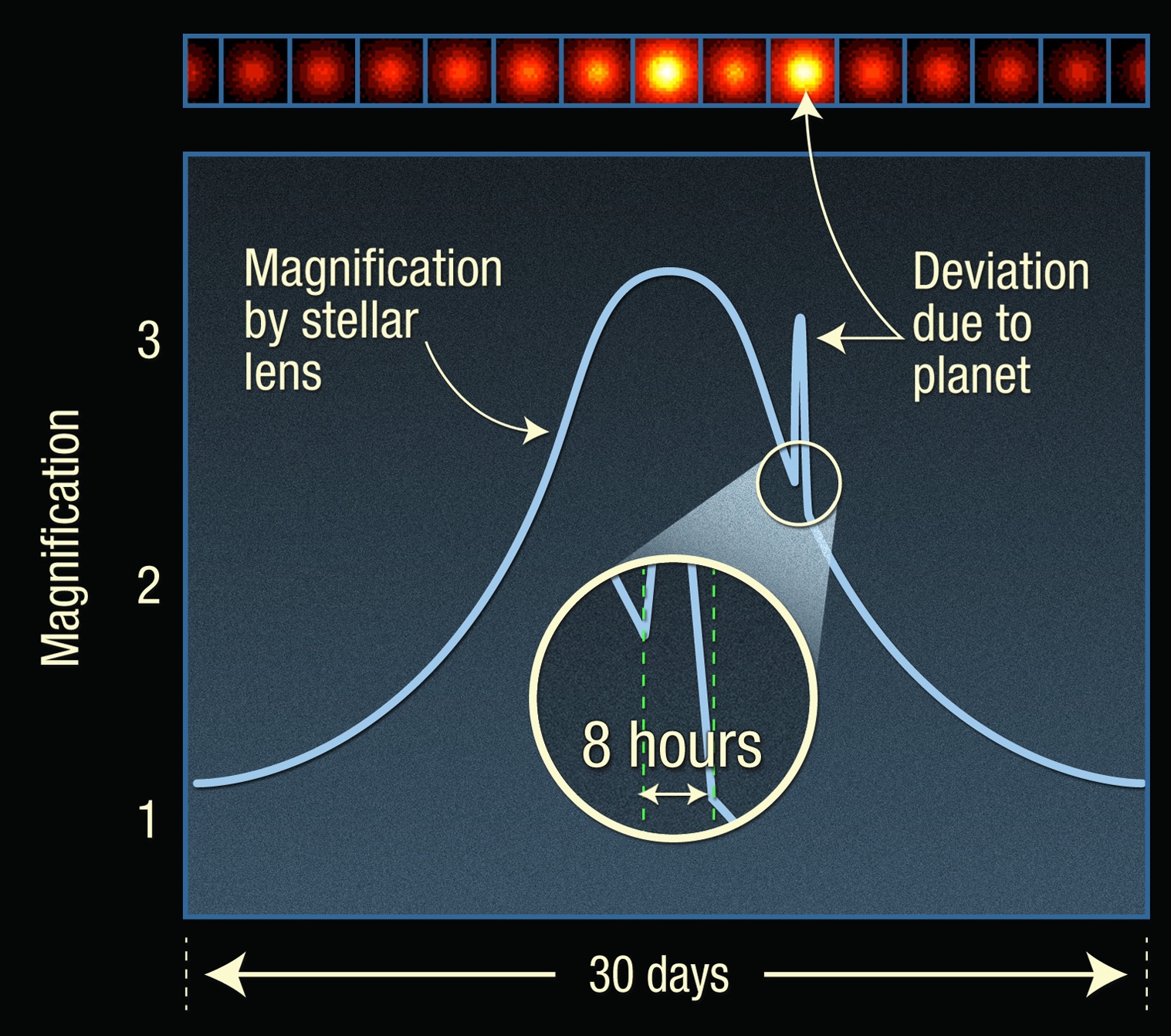
A schematic graph of a large pulse and a smaller narrower pulse superimposed on top.

An illustration of how exoplanets are found via microlensing. The broad first bump is caused by the host star magnifying the light from a background star; the narrow second bump is caused by the planet acting as a lens as well. “Free-floating” planets create only one bump. [Adapted from NASA, ESA, and A. Feild (STScI)]

The idea that there are more free-ranging Neptunes than stars is unsettling, and astronomers aren’t yet sure how this many planets ended up so isolated. It’s possible that these objects simply formed disconnected from any planetary system, but it’s unclear how something so small could collapse from the interstellar clouds that usually produce stellar-mass objects. It’s also possible that the planets formed around stars in the usual way, only to be later kicked out by some violent dynamical process — but this would either require too much time or too many giant planets capable of ejecting the lower-mass ones.

However, new research by Sam Hadden (Canadian Institute for Theoretical Astrophysics) and Yanqin Wu (University of Toronto) presents an alternative idea: what if at least some of these free-floating planets aren’t fully on their own, but instead remain estranged but weakly bound to their parent stars?

Simulated Scattering

Two celestial objects need to align nearly perfectly in order to create a microlensing pulse that we can detect. For an exoplanet orbiting a star, we should observe two of these pulses: one when the host star drifts in and out of alignment with a background star, and one when the nearby bound planet does the same. In the case of a free-floating planet, there’s only one pulse, and we therefore assume that there is no host star. Hadden and Wu noticed that since the alignment has to be so precise for microlensing to occur, it’s possible that a seemingly free-floating planet is simply widely separated from its host star, and the star managed to dodge the magnification effect. In other words, these planets might not be free floating at all, just on wide and eccentric orbits.

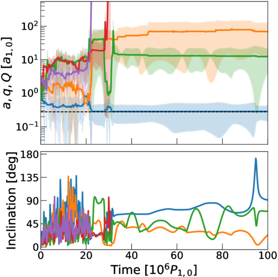
A two-panel plot showing how the semimajor axis and inclination of 5 planets evolve over time.

The orbital evolution of a five-planet system that undergoes planet–planet scattering. Each line represents one planet; note that in the end two are ejected, two end up on wide detached orbits, and the fifth ends up on a tightly bound inner orbit. Click to enlarge. [Hadden & Yu 2026]

The researchers decided to test whether it’s possible to create these kinds of orbits via a known dynamical process called planet–planet scattering. As the name implies, during this process, planets that begin on orderly orbits around their parent star undergo a dramatic rearrangement as they jostle each other around through gravitational interactions. The researchers created two types of simulations: one with a collection of equal-mass planets, and another in which one planet dominates over a brood of smaller ones. After setting up the systems, they let the “dynamical havoc” proceed for a few hundred million years, then surveyed the aftermath.

They found that both types of simulations readily created the “detached” objects needed to mimic free-floating planets. In fact, the most common outcome was for two or three planets to be bullied into far-out orbits by a planet that then plunges onto a tight inner orbit extremely close to the star.

Though the authors caution that this process likely doesn’t explain all of the free-floating planets observed to date, this is an exciting model that would dramatically lower our estimates of the number of Neptunes roaming alone between the stars.

Citation

“Free Floating or Merely Detached?,” Sam Hadden and Yanqin Wu 2026 ApJ 1000 70. doi:10.3847/1538-4357/ae6508

The post Detached but Not Alone appeared first on AAS Nova.
Courtside Seats on Mars

5 June 2026 at 17:00

A photograph of an entire visible hemisphere of Mars.

When the third known object from the galactic space beyond our Sun barreled through the solar system last year, Earth was in a terrible spot to view its flyby. Thankfully, however, a spacecraft that was previously busy mapping Mars took advantage of much better positioning for a closer look.

Cheap Seats

Astronomers have now observed three interstellar objects as they’ve flown through the solar system: 1I/ʻOumuamua, which shocked astronomers in 2017; 2I/Borisov, which followed in 2019 and behaved almost identically to a solar system comet; and now 3I/ATLAS, which was found buzzing toward the Sun in July 2025. As soon as 3I/ATLAS was spotted, pretty much every telescope on the planet took a look. The data swiftly revealed much that intrigued astronomers: while 3I/ATLAS was behaving essentially like a standard comet, its chemistry was nothing like its solar system counterparts, and its coma and dust outflow were strangely shaped. Among other oddities, it seemed to counterintuitively have a dust tail that pointed toward the Sun.

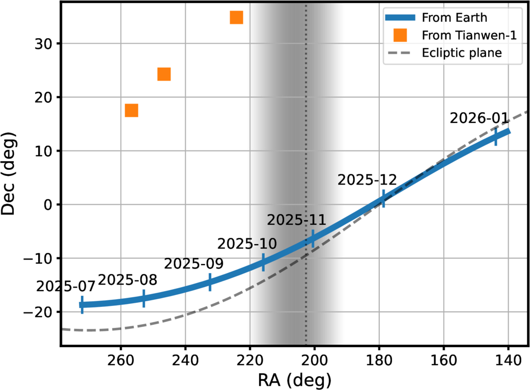
A plot showing that Earth-based observations could only get as best a 20-degree out-of-plane view, while Mars-based observations could get up to nearly 40.

3I/ATLAS’s path across the sky as seen from Earth versus the clearer line of sight from Mars. The shaded region represents the times where the comet was too close to the Sun for viewing. [Xin Ren et al. 2026]

Unfortunately for astronomers, 3I/ATLAS didn’t make it easy for them to study the shape of its coma. Thanks to a cosmic coincidence, the interstellar visitor was traveling almost perfectly within the plane of our solar system, and Earthbound observers were often limited to an edge-on view of its tail. Even worse, 3I/ATLAS looped around the back of the Sun from our perspective, meaning no one on the planet could observe the comet for a few weeks in the fall. This led a group of astronomers to consider their assets that are farther from home.

Better View from Mars

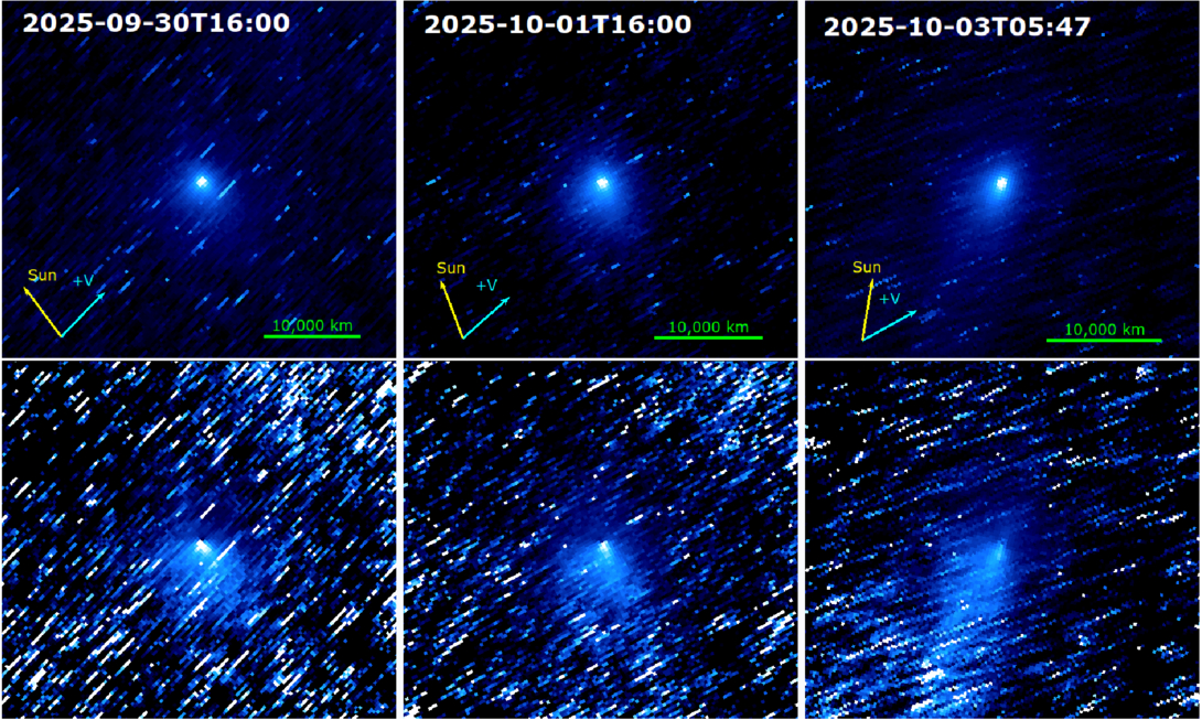
The Tianwen-1 spacecraft, which entered Martian orbit in early 2021 and has been diligently mapping the Red Planet ever since, has a high-resolution camera that’s normally pointed at the planet’s surface. By spinning the spacecraft around, a team of researchers led by Xin Ren (National Astronomical Observatories, Chinese Academy of Sciences) repurposed the camera to act as a small telescope when 3I/ATLAS flew by. In another cosmic coincidence, 3I/ATLAS happened to pass very near Mars last fall, and this close approach gave Tianwen-1 a great out-of-plane view of the coma. The orbiter managed to capture 57 images of 3I/ATLAS over three days last fall, representing China’s first-ever observations of an object from an asset in deep space.

Multi-panel photographs of a comet against a background of streaked stars.

Stacked images of 3I/ATLAS from the Tianwen-1 orbiter across three epochs; the tail’s apparent shape shifts as the viewing geometry changes. Click to enlarge. [Xin Ren et al. 2026]

The team took full advantage of the great view and leveraged the spacecraft’s unique perspective to extract some intriguing results. By tracking how the gentle pressure of sunlight nudged the escaping grains, the researchers found that the coma is dominated by surprisingly large dust. With an average size of hundreds of microns across, the dust is more like coarse sand than smoke, and they found that it ambles away from the comet at just 3–10 meters per second. All told, 3I/ATLAS was shedding dust at roughly 1,000 kilograms every second. The big grains may be a fingerprint of a cold, distant birthplace: models suggest such grains collect in the frigid outer reaches of planet-forming disks, hinting that 3I/ATLAS was forged far from its parent star before being flung into the dark.

As new surveys begin to turn up interstellar interlopers more often, this improvised observation makes a tidy point: the spacecraft already scattered across the solar system can double as a fleet of opportunistic comet-watchers, each offering a view we simply can’t get from home.

Citation

“Interstellar Object 3I/ATLAS Observed from Mars by China’s Tianwen-1 Spacecraft,” Xin Ren et al 2026 ApJL 1003 L10. doi:10.3847/2041-8213/ae61b3

The post Courtside Seats on Mars appeared first on AAS Nova.
Playing Pool with Planets

22 May 2026 at 17:00

artist's impression of hot Jupiter exoplanets

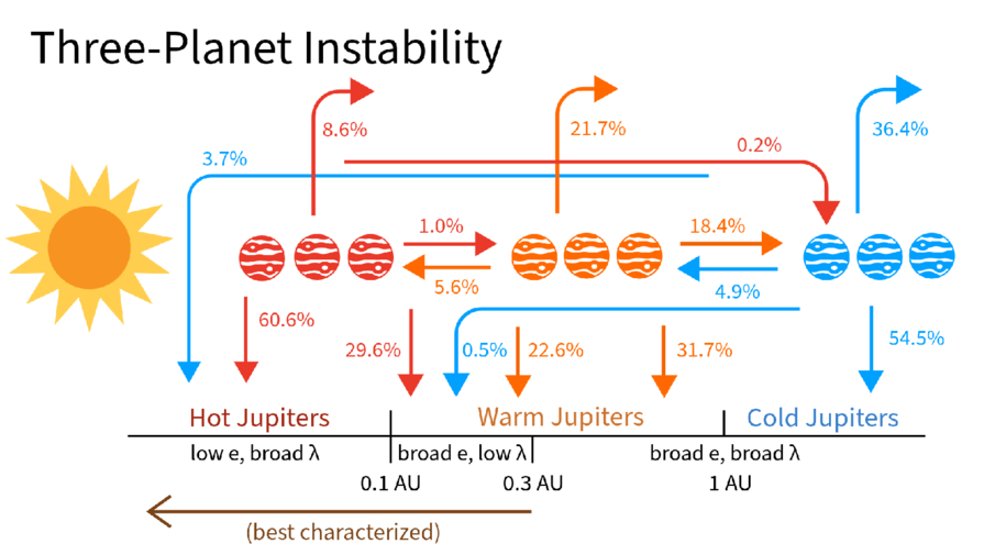
Each Jupiter-size planet in the galaxy falls into one of three distinct categories: hot, warm, or cold. A new study suggests that despite the apparent differences between these populations, they may have all formed from the same underlying dynamical process: a game of pool played at planetary scales.

A Diversity of Jupiters

Though our solar system has only one Jupiter-size planet, elsewhere in the galaxy we have found three different species of these massive gas giants. Cold Jupiters closely resemble their namesake and orbit far from their host stars; hot Jupiters are the opposite and are found whipping around their stars on extremely close-in orbits. In between these are the warm Jupiters, which tend to orbit in the intermediate space between 0.1 and 1.0 au.

A rendering of a star with lots of spots and flares with a planet in the foreground.

An artist’s depiction of a hot Jupiter. These planets orbit extremely close to their host stars, but likely got to their locations by scattering inward from more distant orbits. [NASA/JPL-Caltech]

Though these three populations are defined by their orbital distances, they differ from each other in other ways as well. For example, hot Jupiters almost never have nearby companions; if there are any other planets circling the same star, they’re usually far-out cold Jupiters. They can also orbit in pretty much any direction, including opposite the direction of their star’s spin, and are usually on perfectly circular orbits. In contrast, warm Jupiters often have friends nearby, are much more aligned with their stars’ spins, and can have modest eccentricities.

Given these differences, it’s often thought that each of these populations arrived at its current location through different dynamical processes and that the history of the warm Jupiters is likely quite different from the history of the hot Jupiters. However, a new study led by Julia Esposito (Georgia Institute of Technology) has proposed an alternative view. Maybe these populations, though they appear different now, were all created by the same process: planet–planet scattering.

Virtual Planetary Billiards

A cartoon of Jupiters at different distances from the sun with labelled arrows flowing inwards and outwards from each.

A schematic showing where different planets ended up as a function of where they scattered from during their evolution. Click to enlarge. [Esposito et al. 2026]

Esposito and collaborators set up 1,500 virtual planetary systems with three massive planets each, then simulated how the orbits evolved before probing the final configurations. In crucial contrast to previous simulation studies, the team initialized their Jupiters across a range of different distances and included the effects of tides sapping energy from orbits of planets that got too close to their host stars.

At the end of the simulation, the team surveyed the digital carnage. Almost every virtual system ended with only two planets after either ejecting one away from the star or having two planets collide. But, remarkably, the remaining two-planet systems looked tantalizingly similar to what we actually observe, with a mix of hot, warm, and cold Jupiters. Even more exciting, the end populations were highly correlated to where the violent scattering event took place.

For example, the warm Jupiters were almost all produced by “warm scattering” simulations, where the scattering took place between 0.1 and 1.0 au. The planets that survived the simulations and ended up as warm Jupiters matched all of the properties of the real warm Jupiter population: they had nearby companions, were moderately eccentric, and were mostly aligned with their stars. The hot Jupiters, meanwhile, were almost all produced by “cold scattering” events where the flybys happened far from the star and resulted in one planet hurtling inwards. These also matched all of the observed properties of real hot Jupiters.

The researchers concluded that planet–planet scattering can produce both the warm and hot Jupiter populations so long as you let the planets scatter from a variety of different distances. This exciting theoretical insight, if correct, would mean that astronomers could stop searching for different pathways to create each population. Happily, this model also provides testable predictions, and the authors lay out how the theory could be supported or disproven with additional data. Through virtual experiments like these, astronomers continue to build up an understanding of how the wide range of planetary architectures observed across the galaxy came to be.

Citation

“Unified Formation Channel of Hot and Warm Jupiters via Planet–Planet Scattering,” Julia Esposito et al 2026 ApJL 1003 L3. doi:10.3847/2041-8213/ae61b0

The post Playing Pool with Planets appeared first on AAS Nova.
A New View of the Spectroscopic Universe

8 May 2026 at 17:00

A photograph of a telescope opened at dusk.

The Sloan Digital Sky Survey (SDSS) fundamentally changed the way modern astronomy research is done. This “grand and bold thing” is not frozen in a museum exhibit, however: instead, the SDSS telescopes and team have continued to iterate. The collaboration recently described the fifth generation of this groundbreaking survey in The Astronomical Journal.

Roots in History

Astronomy is now without question a “big data” science. While a lucky few researchers still occasionally travel to distant mountaintops to sojourn with the stars, most astronomers who can describe their work as “observational” rarely ever leave their laptops. Petabytes of historical data, including images, spectra, enormous simulation archives, and more, are available the instant one’s fingers touch a keyboard. As a result, the speed of discovery has increased exponentially, and the barriers to cutting-edge research have dramatically shrunk.

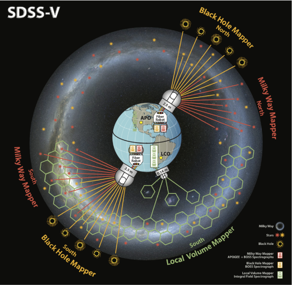
A cartoon of the Earth with three telescopes roughly geographically distributed as they are for the SDSS V survey.

A schematic of the SDSS-V survey facilities and targets. Click to enlarge. [Kollmeier et al. 2026]

While no paradigm shift can be pinned to an exact date, astronomy’s turn towards the data-rich era arguably began in 1998 when SDSS first began collecting data. This was among the first of the “industrial” surveys that observed large swaths of the sky with electronic detectors and used automated pipelines for bulk data processing. In the years since, larger robotic telescopes have begun to mimic the SDSS strategy of “mowing the sky.” The latest of these successors, which itself may usher in another paradigm shift in terms of data volume and availability, is the soon-to-begin Legacy Survey of Space and Time at the Vera C. Rubin Observatory.

While SDSS’s twin 2.5-meter telescopes (one in New Mexico and one in Chile, allowing the survey to observe the entire sky) are dwarfed by Rubin’s 8-meter mirror, there is still thrilling science to be done with these moderate-sized observatories. This is especially true after a series of upgrades to the spectrographs and thanks to a deep expertise in not only survey-style science, but also in project management and survey planning. In 2021, in the middle of COVID-19 delays and distancing requirements, the team began upgrades to their existing facilities and construction of a brand new telescope to kick off the latest survey, SDSS-V.

The Next Generation

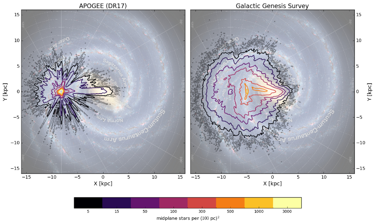
A two-panel figure showing top-down views of the milky way galaxy with different density contours overlaid.

The density of target stars for the SDSS-V survey compared to a previous spectroscopic survey. Click to enlarge. [Kollmeier et al. 2026]

In a wide-ranging publication that references not only astronomy research articles but also Plato, the Bhagavad Gita, an Egyptian tomb, and Tolstoy, the large collaboration describes that this latest survey is divided into three parts: the Milky Way Mapper, the Black Hole Mapper, and the Local Volume Mapper. The preexisting telescopes, which are outfitted with hundreds of tiny robots that can swivel fiber optic cables into place to collect spectra of up to 500 objects at a time, will handle the first two of these “mappers.” A brand-new facility in Chile that’s specifically designed to map the structure of nearby gas will handle the last mapper. Instead of aiming the fibers at a known star or galaxy, this telescope will instead collect a spectrum for every point across an area the size of the full Moon with every exposure.

By the end of the survey, SDSS-V will have collected optical and near-infrared spectra for roughly 6 million objects spread across the whole sky, as well as time-series spectra from about a million of these sources. This dataset, which is unprecedented in both its spatial and temporal coverage, will allow researchers to probe questions ranging from how quasars evolve over time to how commonly young stars have brown-dwarf companions. Long since SDSS initiated the era of industrial survey astronomy, this latest publication shows how the survey continues to lead the way.

Citation

“Sloan Digital Sky Survey. V. Pioneering Panoptic Spectroscopy,” Juna A. Kollmeier et al 2026 AJ 171 52. doi:10.3847/1538-3881/ae0576

The post A New View of the Spectroscopic Universe appeared first on AAS Nova.
How Galaxies Grow Up

24 April 2026 at 17:00

JWST unfolded against a black background.

How do galaxies grow? A massive survey from JWST can help astronomers answer that fundamental question about galaxy evolution.

Time Machines

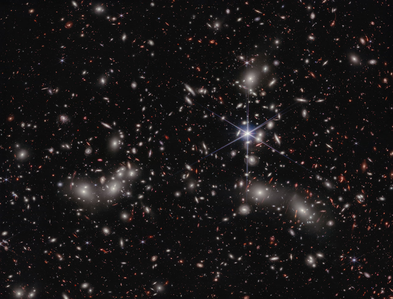
A photograph of thousands of galaxiesin one frame.

An image taken by JWST’s NIRCam instrument, the primary instrument behind the COSMOS-Web survey, of Pandora’s Cluster. Click to enlarge. [NASA, ESA, CSA, Ivo Labbe (Swinburne), Rachel Bezanson (University of Pittsburgh); Image Processing: Alyssa Pagan (STScI)]

When astronomers look into the night, they are greeted by a sky full to bursting with galaxies. But immediately after the Big Bang, none of these grand structures could have existed in our universe: all of the matter was too hot and dense to collapse into the whirlpools and ellipses we see today. We know that it took time for dark matter to collapse into halos, for gas to cool and fall into those halos, and even more time for those halos to merge together and galaxies to form. However, quantifying that story is tricky. How long did it take for the gas to cool and collapse? How often did small galaxies merge? How did the birth and death of stars play into all of this?

One way astronomers could go about answering these deep, fundamental questions in galaxy evolution would be to look at many galaxies spread across different distances. Famously, since the speed of light is fairly slow (cosmically speaking), we can only see distant objects as they appeared in the past. (This is why any aliens looking toward Earth from 65 million light-years away — from within the Virgo Cluster, perhaps — would see our planet as it was when dinosaurs roamed free.) In principle, then, by looking at a progression of galaxies farther and farther away, astronomers could convert these still images into a sort of movie of how typical galaxies look moving further and further back in time.

Seeing Red

There is a complication to this strategy, however. The farther away an object is, the more the light it emits is stretched towards redder wavelengths. As a consequence, any telescope designed to detect visible light won’t see anything; to take pictures of these galaxies, we need to build detectors that are specifically sensitive to stretched-out, near-infrared light.

This is one of the primary reasons that JWST was designed, constructed, and flung into space. It was purpose-built to collect and analyze near-infrared light from distant galaxies, and now after several years of observations and data crunching, astronomers are finally getting some answers to those fundamental questions.

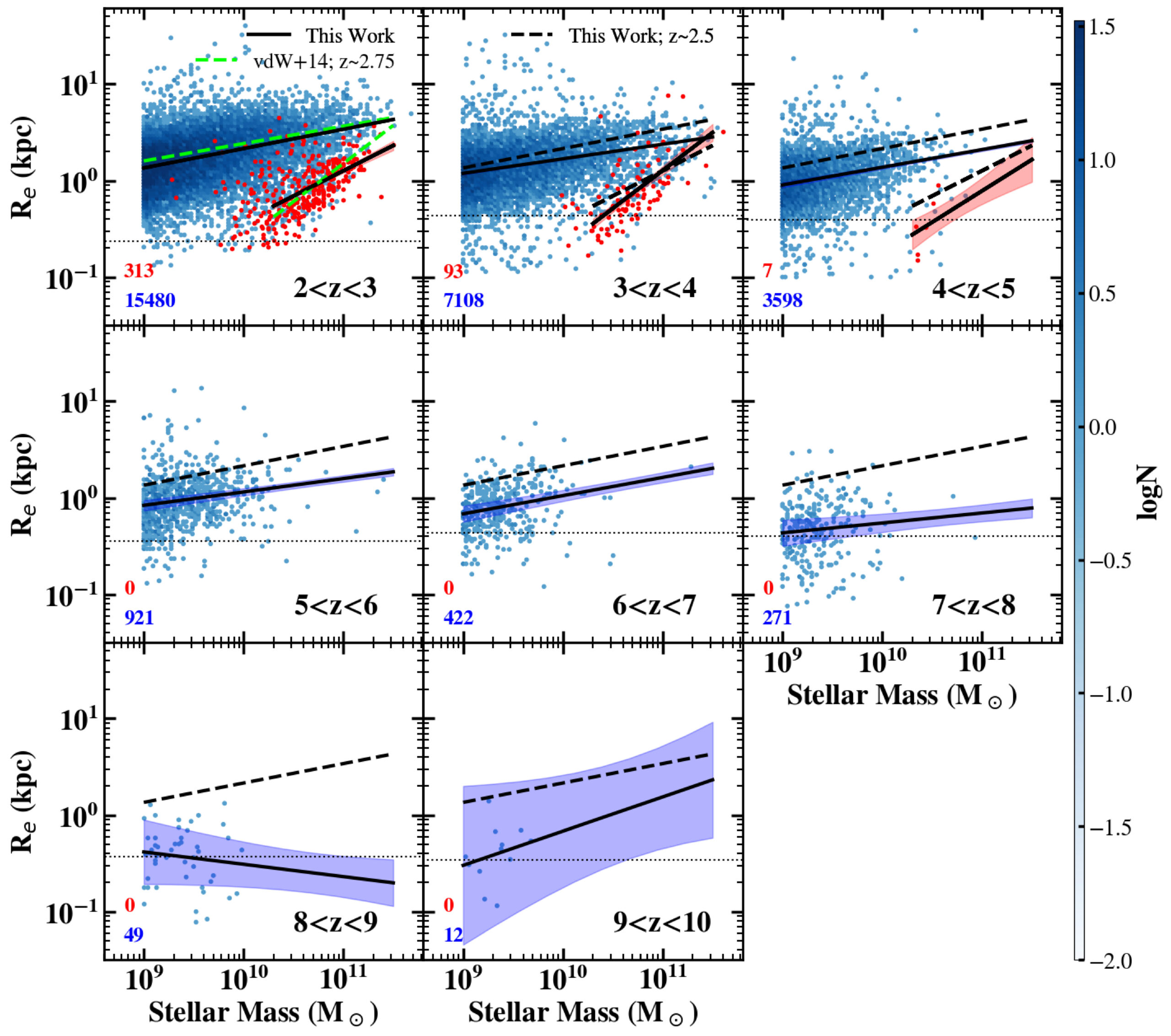
The results of how galaxies’ masses relate to their total size in different redshift bins. Click to enlarge. [Yang et al. 2025]

A Massive Survey

Recently, a team led by Lilan Yang, Rochester Institute of Technology, released their analysis of one of the earliest and largest surveys JWST has undertaken, a program called COSMOS-Web. The researchers mined a patch of sky about the size of the full Moon and extracted more than 30,000 distant galaxies, most of which had never before been seen by human eyes. They measured the brightness and size of each one and grouped them according to their redshift (a proxy for their distance) and whether they were actively forming stars or not.

The team found that, unsurprisingly, galaxies tend to grow over time. Excitingly, however, they also found that for star-forming galaxies, the relationship between a galaxy’s mass and its size is fairly constant for redshifts of z = 2–8. The scaling law between them also nicely matches up with measurements taken by the Hubble Space Telescope at smaller redshifts. Beyond that, though, for redshifts of z = 8–10, it’s possible that the scaling changes, though the authors emphasize that their sample is much smaller in these distant bins.

While more data are needed to confirm whether the youngest of these galaxies grow at a different pace than their later counterparts, we can be comforted that studies like this represent just our very first peek into a whole new era of galactic evolution, and that many more insights are sure to come as JWST keeps snapping images.

Editor’s Note: This article previously contained an error relating to the distance at which aliens would see Earth as it was when inhabited by dinosaurs. This error was corrected on 4 May 2026.

Citation

“COSMOS-Web: Unraveling the Evolution of Galaxy Size and Related Properties at 2 < z < 10,” Lilan Yang et al 2025 ApJS 281 68. doi:10.3847/1538-4365/ae0e1b

The post How Galaxies Grow Up appeared first on AAS Nova.
Enhancing the Sharpest Images

15 April 2026 at 17:00

The Submillimeter Array at the summit of Maunakea in Hawaiʻi.

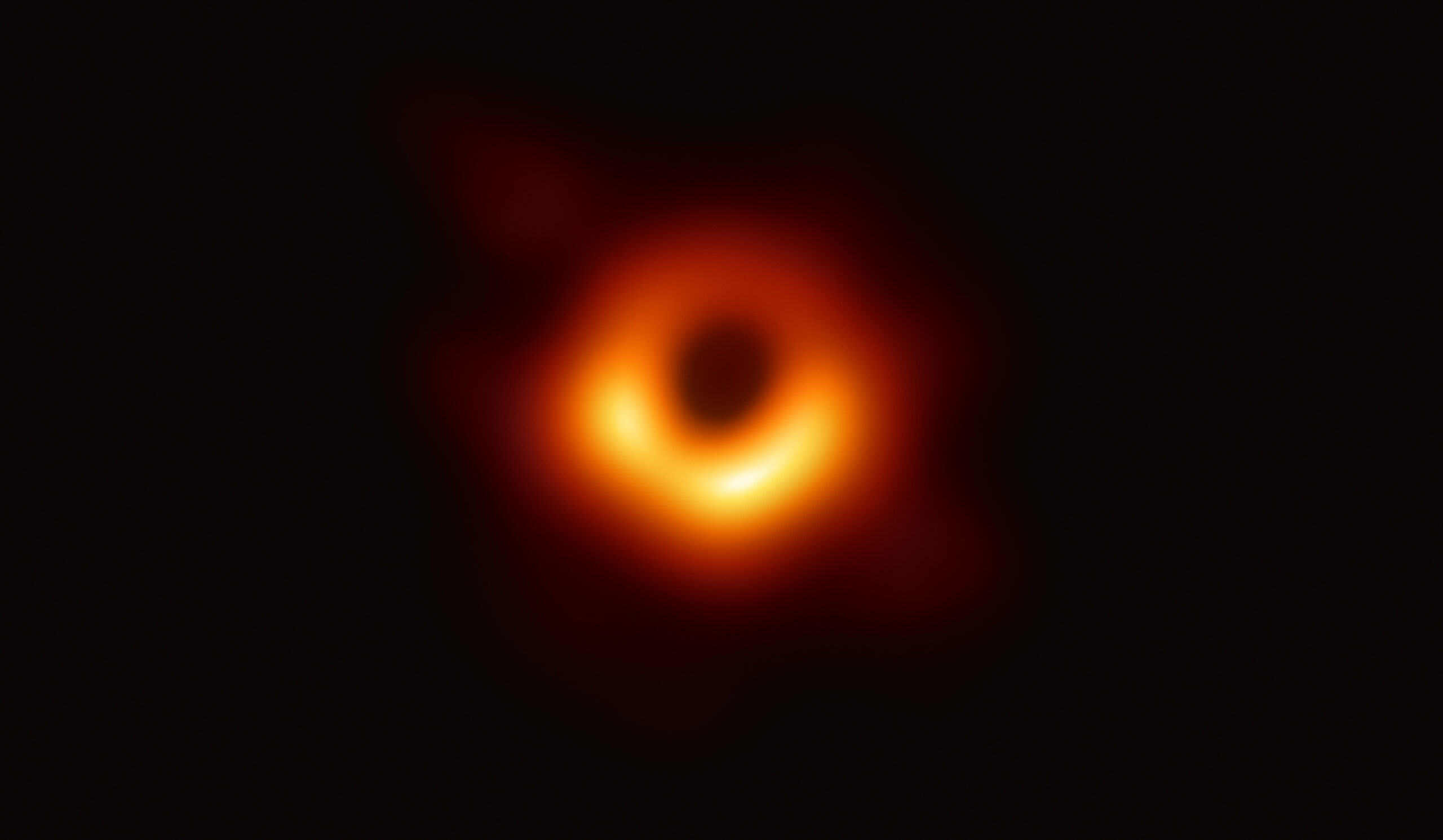
The Event Horizon Telescope (EHT), the facility that delivered humanity’s first-ever picture of a black hole, can produce some of the sharpest images in all of astronomy. But turning the EHT’s raw data into images is a complex process involving messy statistics and powerful algorithms. Recent work presents a potential upgrade to that process: for the first time in long-baseline interferometry, it may be possible to model everything everywhere all at once.

The Hardest Eye Test

The EHT has some of the sharpest eyes in all of astronomy. With its effective resolution of just 20 microarcseconds, in principle you could use it to read a newspaper in New York while sitting at a cafe in Paris. But this planet-spanning instrument (it relies on data from radio telescopes on four continents) doesn’t snap pictures like an ordinary camera. Instead, each pair of telescopes measures something called an “interferometric visibility,” which is related to a single Fourier component of the actual underlying image.

A photograph of an orange ring surrounding a dark center.

The first image of a black hole, constructed from Event Horizon Telescope data taken in 2017. [EHT Collaboration; CC BY 4.0]

Combining these components into an image is a process fraught with assumptions and modeling choices. Since the EHT doesn’t have an infinite number of telescopes, each measurement can be mapped to infinitely many images. This forces researchers to choose how to “regularize” this space of images to select one best picture. Making things harder, they also must contend with all the typical issues of real-world data collection. Each telescope has slight calibration errors, and every data point is affected by weather and temperature-dependent processes.

Typically researchers break the problem down into several stages: first calibrate the data, then regularize and construct the best-fitting image, then analyze that image to constrain the actual physics you care about like the width of the ring surrounding a black hole. This is how the original EHT publications went about their groundbreaking work on the now-iconic glowing ring around the supermassive black hole in the galaxy Messier 87 (M87*).

A New Approach

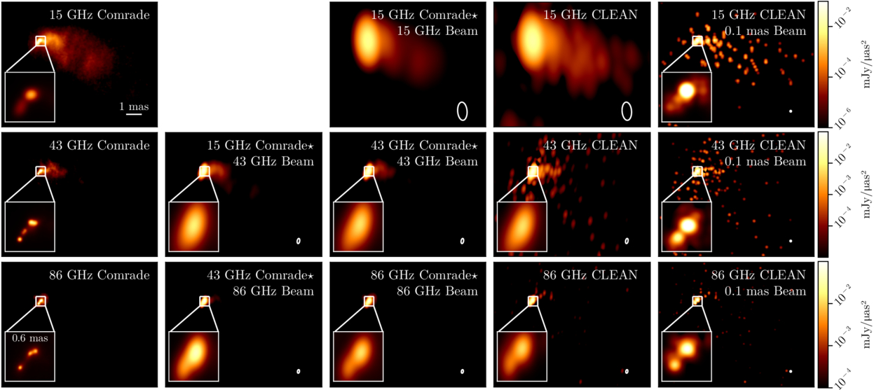
Recent work led by Paul Tiede (Black Hole Initiative at Harvard University) suggests an alternative process. Instead of separating the stages of analysis as described above, the team demonstrated that one could fit everything simultaneously in a framework they call hierarchical interferometric Bayesian imaging, or HIBI.

A multi-panel plot of images of an orange blob with a tail. All images are very similar.

A comparison of the new HIBI technique (referred to as “Comrade” here) and a traditional algorithm called CLEAN. Click to enlarge. [Tiede et al. 2026]

By fitting all parameters that go into an image together, the method doesn’t select one “best” image. Instead, by allowing the pixel-by-pixel intensities, calibration parameters, and underlying physics to inform one another during inference, HIBI explores the full range of images consistent with the data. This prevents the degeneracies that plague the traditional approach, where image and calibration estimates can trade off against each other in misleading ways. The team validated HIBI on synthetic data mimicking the EHT’s 2017 setup, showing that it reliably recovered a range of source shapes with well-calibrated uncertainty estimates.

Even more exciting, the team demonstrated that it’s possible to skip the image construction step altogether and go straight to the science. By fitting parameters describing the physics underlying a scene, the team was able to constrain the width of the ring around M87* without any reference to a picture. They predict that this technique could be crucial for extracting information when future instruments like the Next Generation Event Horizon Telescope observe more distant black holes that are only marginally resolved. Though we’ll likely have to wait years for these next-generation telescopes, work like this ensures that astronomers will be able to squeeze as much science from them as possible once these new facilities are ready.

Citation

“Hierarchical Interferometric Bayesian Imaging,” Paul Tiede et al 2026 ApJ 997 262. doi:10.3847/1538-4357/ae2749

The post Enhancing the Sharpest Images appeared first on AAS Nova.

An Impostor Explosion

27 March 2026 at 16:00

A rendering of two purple jets streaming away from a central explosion.

Over many centuries of observing the night sky, astronomers have found only a single visible afterglow of a collision between neutron stars. For a few days in the summer of 2025, it seemed like observers may have found another of these treasured but elusive prizes; unfortunately, the promising candidate turned out to be a supernova in disguise.

A Rare Prize

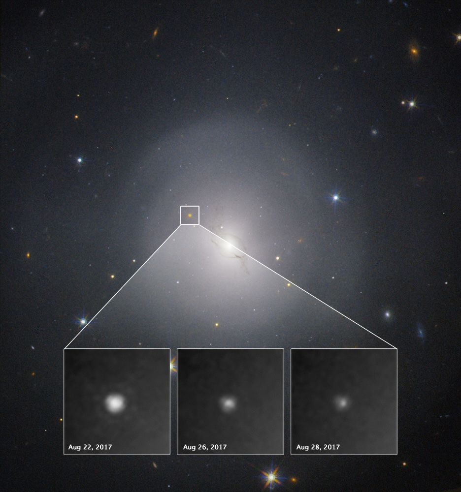
kilonova as seen by Hubble

These images from the Hubble Space Telescope show the fading light of the kilonova associated with the gravitational wave event GW170817. [NASA and ESA Acknowledgment: A. Levan (U. Warwick), N. Tanvir (U. Leicester), and A. Fruchter and O. Fox (STScI)]

When two neutron stars (the ultra-dense remnants of massive stellar explosions) spiral together and collide, the cataclysm is energetic enough to release strong gravitational waves, forge heavy elements, and briefly glow across the electromagnetic spectrum. These events are called kilonovae, and they’re quite rare; while we may have detected a handful at high energies, there is only one event for which astronomers managed to record both gravitational waves and an optical transient.

That one kilonova, found back in 2017, taught astronomers much about how heavy elements are formed and left the scientific community hungry for more data. Since then, each time a gravitational wave detector like LIGO reports that it may have spotted a neutron star merger, telescopes across the world scramble to look in the probable region of the sky, hoping to find the short-lived electromagnetic counterpart.

Too Good to Be True

On 18 August 2025, the LIGO/Virgo/KAGRA collaboration sent out an alert that it may have detected a neutron star–neutron star merger. The odds that their signal was real weren’t great, and the researchers gave it just a 29% chance of being a genuine astrophysical signal. Still, given the potential payoff of finding the next kilonova, several telescopes quickly began searches for the optical counterpart. The gravitational wave signal suggested that the event likely came from a curved patch of sky delightfully referred to as the “northern banana,” and after trawling that region for a few nights, astronomers hauled in 47 new transients. Any one of these could have been the kilonova, and all of them received extensive follow-up observations.

A team led by James Gillanders (University of Oxford) recently summarized some of these follow-up observations carried out with the Pan-STARRS and ATLAS telescopes. In the initial exciting few days after the alert went out, one candidate transient stood out as the most promising. Named AT2025ulz, it was first spotted by the Zwicky Transient Facility and initially started fading rapidly and changing colors, just as models of kilonovae predict. For four days, it seemed like the world may have witnessed its second-ever kilonova. But then the telescopes began their fifth night of observations.

Supernova Unmasked

A scatter plot showing a rapidly fading, then reversing and spiking, light curve.

The light curve of SN2025ulz. Note that the source appeared to grow brighter again after about 5 days. Click to enlarge. [Gillanders et al. 2025]

The light curve of AT2025ulz, after fading steadily in the preceding days, suddenly turned upwards; in other words, whatever was causing the transient got brighter. Models of kilonova evolution predict no such brightening, but Type IIb supernovae are known to follow just this behavior. AT2025ulz showed itself to be another run-of-the-mill stellar explosion, not the sought-after fireworks of two neutron stars slamming together.

Frustrating as this particular result may be, the effort was far from wasted. The team could use their non-detection of the true kilonova to place limits on its timing and peak magnitude, assuming it existed in the first place. And, as gravitational wave detectors grow more sensitive and alerts like this more common, hindsight will likely frame this scramble as a dress rehearsal for an ultimately successful kilonova recovery effort. Until then, astronomers will keep searching, and will keep their guard up against cosmic impostors.

Citation

“Pan-STARRS Follow-Up of the Gravitational-Wave Event S250818k and the Light Curve of SN2025ulz,” J. H. Gillanders et al 2025 ApJL 995 L27. doi:10.3847/2041-8213/ae2125

The post An Impostor Explosion appeared first on AAS Nova.
Jupiter’s Atmosphere Holds Steady

13 March 2026 at 16:00

A close-up photograph of Jupiter. Dramatic cloud bands encircle the planet, and a large dark shadow of a nearby moon appears at left.

Jupiter’s upper atmosphere is hundreds of degrees hotter than it has any right to be, and for decades astronomers could only study it in brief, seemingly chaotic glimpses. New global maps built from years of observations have finally revealed the big picture — and it is surprisingly calm.

Order from Chaos

Although we’re well acquainted with Jupiter, having sent eight spacecraft on close passages and lived with it dominating the night sky for millennia, some of its simplest characteristics continue to puzzle us. For example, high above Jupiter’s cloud bands, temperatures exceed 800 K — far hotter than we’d expect given the meager sunlight that reaches that distance. Astronomers have long suspected that this excess is deposited by energy from the planet’s brilliant polar auroras, but previous observations provided only localized, sporadic snapshots that collectively painted a confusing picture of an ever-changing landscape.

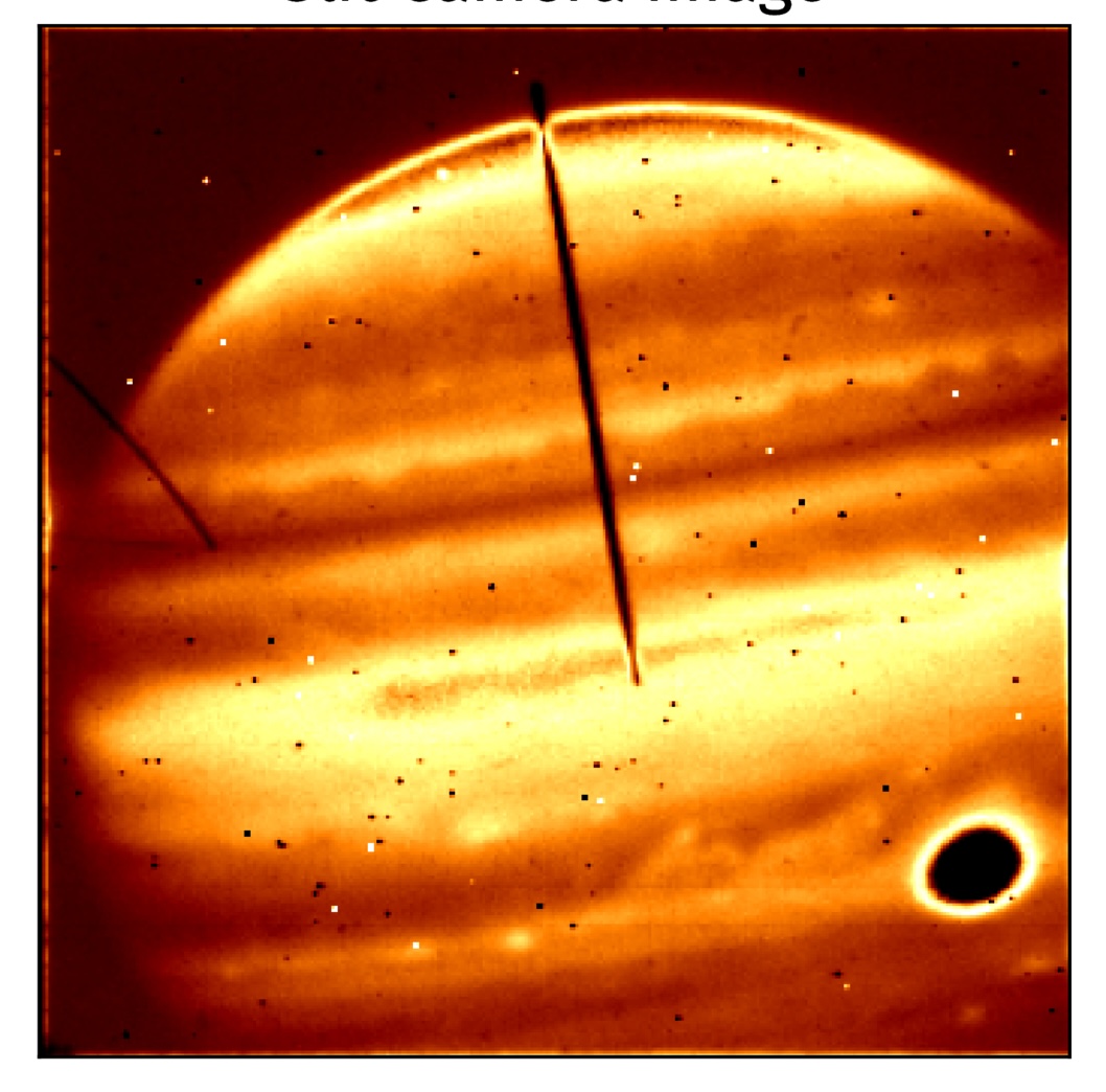
A photograph of Jupiter seen in red/orange false color with a dark stripe down the middle.

Jupiter as seen by the slit camera on the Keck telescope during one of the team’s observations. The spectrograph slit is the dark vertical band stretching from the equator to the north pole, and the Great Red Spot appears in black at the lower right. [Adapted from Roberts et al. 2026]

To truly understand how Jupiter’s upper atmosphere got so hot and whether it was actually changing over time, astronomers needed to construct a global, comprehensive map — and then do so repeatedly over several years and look for any changes. A team led by Kate Roberts (Boston University) has now assembled just this sequence using the NIRSPEC instrument at the Keck Observatory. The researchers collected over 175,000 high-resolution infrared spectra across 14 nights from 2022 to 2025; they then processed the massive dataset to extract the emission from a charged form of hydrogen, H3+. This species is a standard natural thermometer that glows at infrared wavelengths, and by mapping the spectra to their corresponding specific locations on Jupiter, the team could construct the first true global maps of Jupiter’s upper atmospheric temperature, density, and radiance.

Consistency is Key

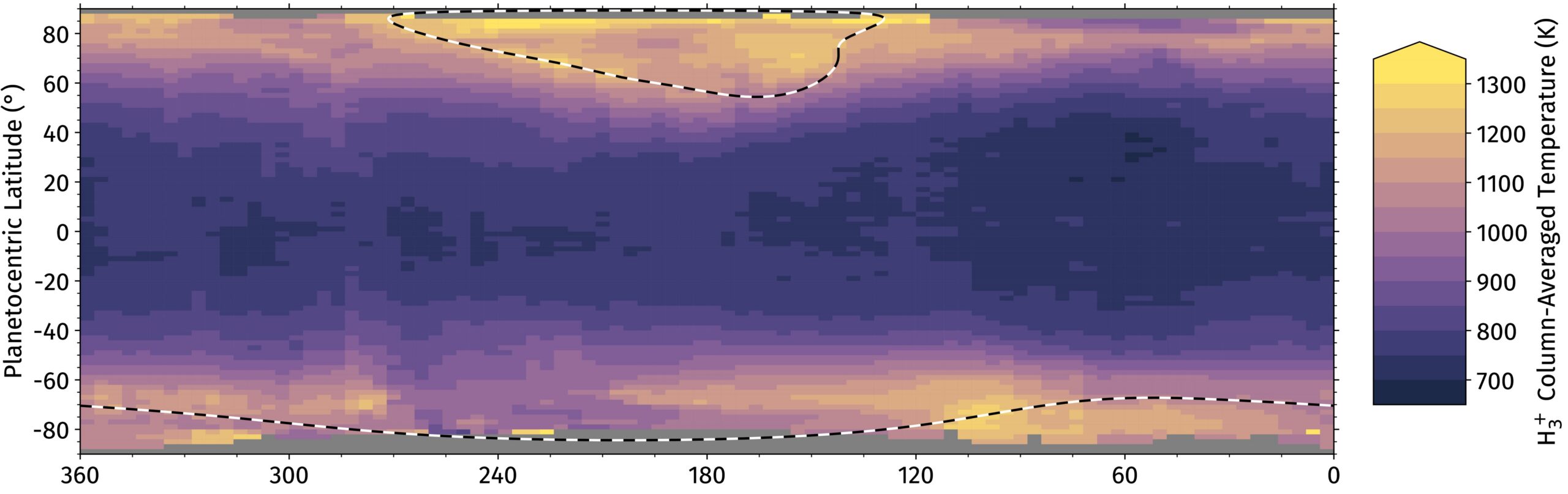
A look at how the maps evolved over time revealed striking order: the spatial patterns remained nearly constant, and the temperatures barely changed even over years. In general, the team noted that temperature decreases smoothly from the auroral regions near the poles (~1,150 K) to the equator (~750 K) at every longitude, and that although there is some night-to-night temperature variation, things stay remarkably steady over the years-long baseline.

A 2D heatmap with longitude on the bottom axis and latitude on the vertical axis. There is a general trend towards higher temperatures at higher latitudes.

A map of the average temperature of Jupiter’s upper atmosphere, as measured by the new Keck NIRSPEC data. Click to enlarge. [Adapted from Roberts et al. 2026]

What once “appeared stochastic,” the authors write, “exhibits predominantly spatial rather than temporal variability.” Earlier observations were simply sampling different longitudes at different times, mistaking geography for weather.

The conclusion that the upper atmosphere is complex but steady has implications beyond just Jupiter, as the team notes that JWST has already observed spatial patterns in the temperatures of the upper atmospheres of both Uranus and Neptune. As Roberts and colleagues note, “similar physical mechanisms could give rise to comparably stable structures” on those distant ice giants, meaning this analysis could ground our understanding of the upper atmospheres of giant worlds across the solar system.

Citation

“A Global View of Jupiter’s Upper Atmosphere Through H3+,” Kate Roberts et al 2026 ApJL 998 L13. doi:10.3847/2041-8213/ae3c9b

The post Jupiter’s Atmosphere Holds Steady appeared first on AAS Nova.
Black Holes with a Shared Background

19 November 2025 at 17:00

A rendering of three white stars, two of which are very close together.

What if there was one process capable of creating every type of detectable stellar-mass black hole system? Recent research suggests there might be, and that it involves a triple-star system.

Three Separate Contexts

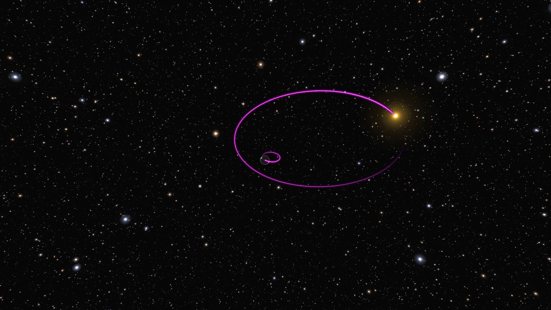
Stellar-mass black holes, or black holes that are at most a few hundred times the mass of the Sun, pop up in a number of different environments in the Milky Way. Astronomers have known since the 1960s that these black holes are the engines behind accreting low-mass X-ray binaries; more recently, researchers at gravitational wave observatories such as LIGO have found pairs of black holes orbiting each other just prior to merging; and, in just the past few years, scientists using the Gaia spacecraft have found black holes on wide, prowling orbits around still-burning stars.

A photograph of a patch of the night sky with two nested purple ovals overlaid.

An illustration of the first black hole discovered with a star on a wide orbit. The black hole moves along the smaller inner ellipse, while its companion star orbits along the wider outer one. [ESA/Gaia/DPAC]

Although each of these scenarios involves a black hole, it’s unclear how exactly these black holes are related to one another, or if they’re related at all. For instance, do low-mass X-ray binaries form the same way as the binary black holes observed with LIGO? Are the wide star–black hole binaries discovered by Gaia destined to eventually merge as two black holes, or are they a separate population altogether?

Recent research led by Smadar Naoz (University of California, Los Angeles) offers a potential answer to this question of relatedness — that each of these situations forms through the same underlying process.

Triples Systems

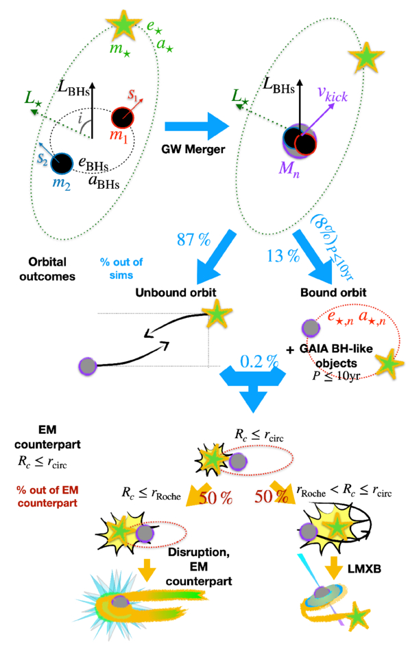
An illustration of multiple stars evolving along different pathways indicated by arrows.

A schematic illustration of how triple-star systems can produce all three types of observable stellar-mass black hole systems. Click to enlarge. [Naoz et al. 2025]

The mechanism Naoz and collaborators describe would work as follows. First, three stars begin their lives all bound together via gravity. Two of these stars orbit each other fairly closely, but the third hangs back much farther away. After the two inner stars burn out and collapse into black holes, they undergo the kind of collision commonly observed by LIGO and merge together. This process gives the resulting larger black hole a “kick,” meaning it goes flying off away from the site of the impact with some new velocity.

What happens next depends on the geometry of the system and the direction of the kick. If the remnant black hole gets shot away from the third star, it might just drift off on its own and leave the star behind. If the kick isn’t too strong, the remnant will remain gravitationally bound to that third star, and the system will eventually look like the star–black hole pairs observed by Gaia. Finally, if the kick sends the remnant toward the third star, some dramatic outcomes become possible: either the black hole starts nibbling on the star and the system becomes a low-mass X-ray binary, or the black hole simply smashes into the star, destroying it completely in a large, flashy explosion paired with a gravitational wave signal.

The authors stress that this mechanism is almost certainly not the only way that these three stellar-mass black hole systems form. However, it is exciting to consider a common thread underlying such seemingly different scenarios, and with upgrades coming to gravitational wave observatories, we can hope for tests of its feasibility in the near future.

Citation

“Triples as Links Between Binary Black Hole Mergers, Their Electromagnetic Counterparts, and Galactic Black Holes,” Smadar Naoz et al 2025 ApJL 992 L12. doi:10.3847/2041-8213/ae0a20

The post Black Holes with a Shared Background appeared first on AAS Nova.
The Sun Left Home in a Hurry

14 November 2025 at 17:00

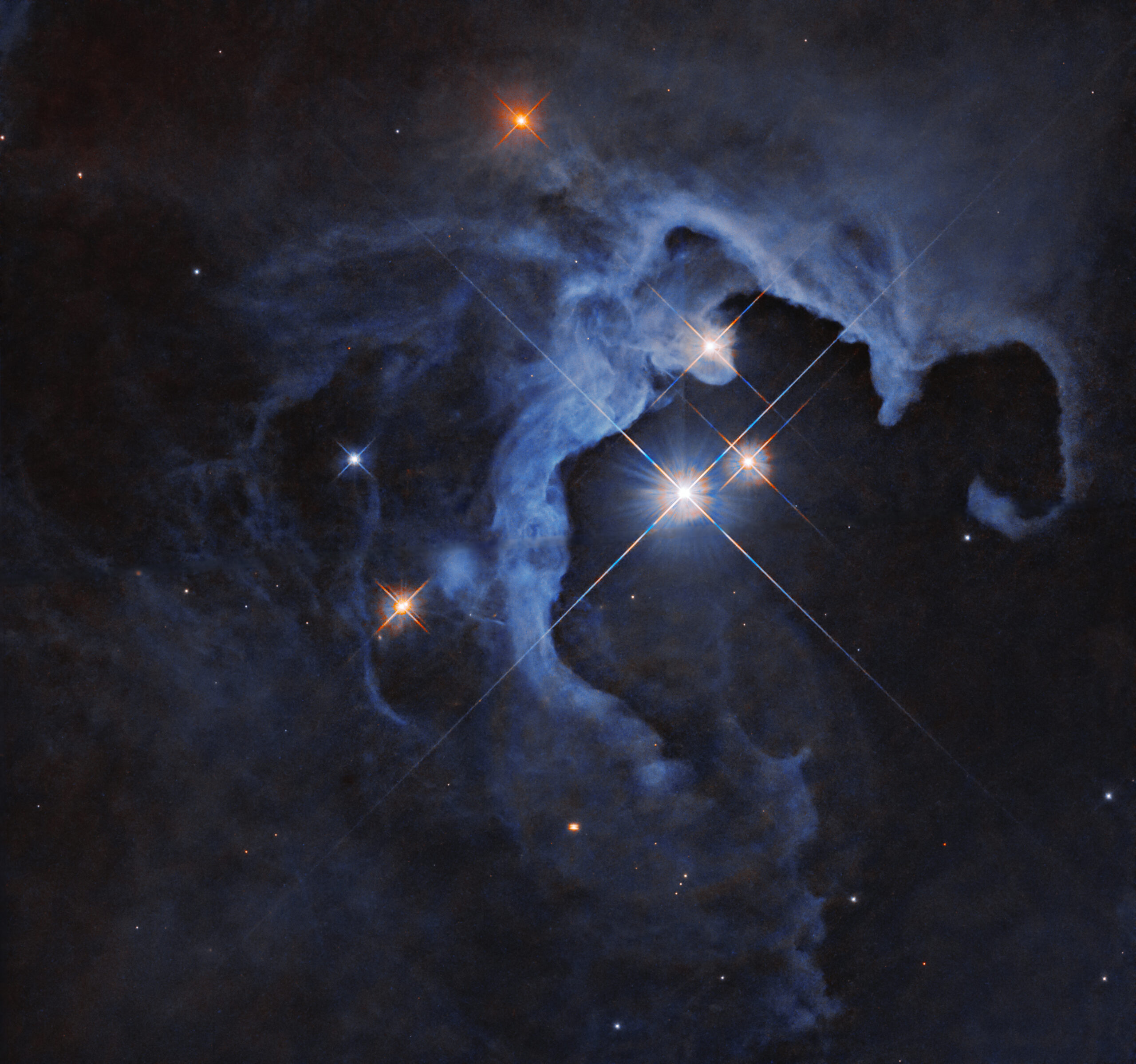
A photograph of a dense knot of stars against a collection of more spread-out stars.

By simulating how the orbits of distant solar system objects were altered by close encounters with other stars early in the Sun’s life, astronomers have placed tight constraints on how long our home star stuck around its siblings after birth.

Born in Batches

Though our Sun currently travels on a solitary trajectory through the galaxy, its earliest childhood was not spent so lonely. Instead, the Sun was likely born as part of a litter of many other stars all collapsing out of the same cloud of precursor gas and dust. As a consequence, its early adolescence was spent in the company of dozens of other young stars, all zipping along on their own paths, destined to drift apart but initially packed close together.

A photograph of three bright stars within a circular cavity of gas.

The Hubble Space Telescope’s view of a collection of young stars still embedded within their natal nebula. [NASA, ESA, G. Duchene (Universite de Grenoble I); Image Processing: Gladys Kober (NASA/Catholic University of America)]

Despite their kinship, these young stars were not kind to one another when they passed nearby. When two stars grow close, the intense gravity of the encounter can severely disrupt their proto-planetary systems, scattering the objects orbiting farthest from their stars and potentially even ejecting some objects altogether. These early years likely left scars on the edges of our solar system that persist even today, billions of years after the early tussles.

Recent research led by Amir Siraj, Princeton University, leverages these scars or their apparent absence to ask the question: given the structure we observe in the outer solar system today, what limits can we place on the number of stars born near the Sun and the amount of time the Sun spent in its birth cluster?

Distance is Power

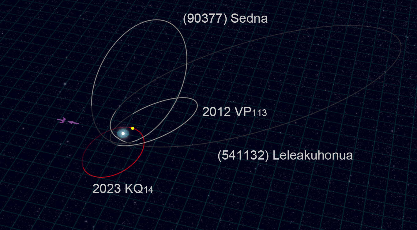
Several authors have asked this question over the past several decades, but Siraj and collaborators added a new twist: instead of studying either the giant planets or the cold classical Kuiper Belt, they instead focused exclusively on the “distant sednoids.” This rarefied collection of only nine known objects includes only the most distant minor planets in our solar system: the sednoids never come within 40 au of the Sun, and they spend much of their orbits beyond 400 au. Interestingly, however, all of them orbit on planes that are fairly aligned with that of the planets, and none ever strays farther than 20° from the ecliptic.

A black background with the sun at center surrounded by several large ovals, each labeled with the name of a minor planet.

An illustration of the orbits for some of the distant sednoids considered in this study. Click to enlarge. [NAOJ]

Through a suite of numerical simulations, Siraj and collaborators demonstrate that this relatively tight distribution of inclinations implies that the Sun couldn’t have been too roughed up on its way out of the cluster. By simulating many different close flybys and their influence on the distant sednoids, the researchers constrained the product of the number of stars in the Sun’s birth cluster and the time the Sun spent there to be less than or equal to 5 billion years per cubic parsec. Assuming a typical cluster density of 100 stars per cubic parsec, this suggests that the Sun cleared out of the densest and most dangerous part of the cluster within just 50 million years.

The authors stress that this conclusion leans on the assumption that the distant sednoids arrived on their extreme orbits essentially immediately, though in fact astronomers aren’t sure exactly how and when these objects ended up on the outskirts of the solar system. If the sednoids were in fact implanted onto their orbits early on, this limit on how long it took the Sun to leave its siblings is by far the strongest to date. With the Vera C. Rubin Observatory poised to discover thousands of new distant solar system objects, it’s likely that the bound will grow even more stringent in the next few years.

Citation

“Limits on Stellar Flybys in the Solar Birth Cluster,” Amir Siraj et al 2025 ApJL 993 L4. doi:10.3847/2041-8213/ae1025

The post The Sun Left Home in a Hurry appeared first on AAS Nova.
Standing on a Sub-Neptune

5 November 2025 at 17:00

A rendering of a blue planet in the foreground and a small bright star in the background.

Astronomers often assume that sub-Neptune exoplanets have magma oceans hiding beneath their atmospheres. New research suggests that this might not always be the case.

Puzzling Type of Planet

In the 30 years since the discovery of the first exoplanet, astronomers have come to appreciate that many of the most common planets in our galaxy look nothing like the worlds in our solar system. One type of planet in particular appears to be ubiquitous despite not appearing in our own cosmic neighborhood: sub-Neptunes. As their name suggests these planets are slightly smaller than Neptune, but still much larger than Earth or what we’d expect from a planet composed mostly of rock.

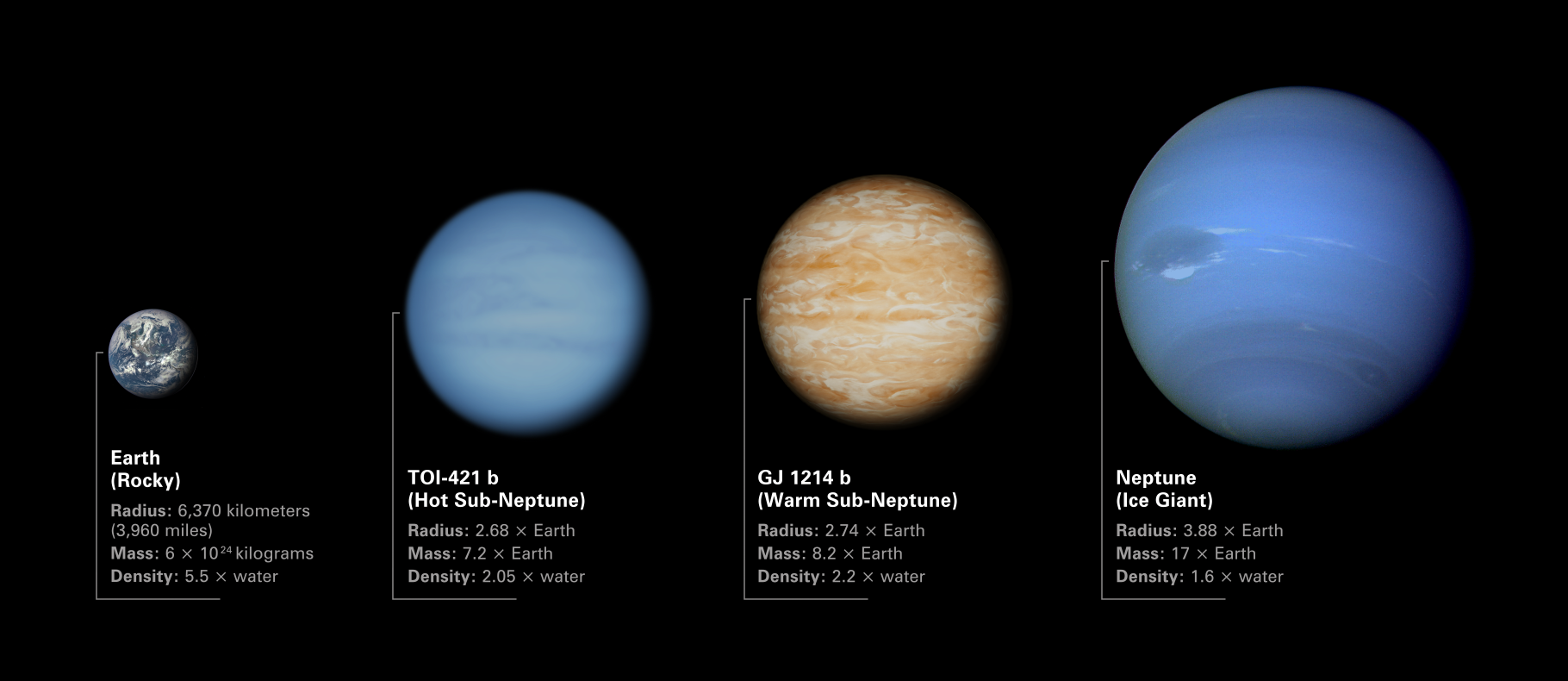
Four planets side by side ordered by increasing size. From left to right, they are Earth, TOI-421 b, GJ 1214 b, and Neptune.

An illustration of how two sub-Neptunes mentioned in this study (TOI-421b and GJ 1214b) compare with planets in our solar system. Click to enlarge. [NASA, ESA, CSA, Dani Player (STScI)]

What sub-Neptunes are made of and how they formed are still mysteries under active investigation by the research community. It is possible that these worlds are mostly rocky and sport puffy, light atmospheres over their surfaces; it’s also possible that these worlds are watery, and that most of their mass comes from heavy, steamy atmospheres. In most cases, though, it’s assumed that the high pressures and temperatures at the surfaces of these worlds foster a permanent, fiery magma ocean.

This key assumption that there’s no solid surface to stand on influences our models about how these planets cool and evolve over time. However, new research led by Bodie Breza (University of Maryland) suggests that this premise might not always be appropriate.

Solid Ground

To test the assumption that every sub-Neptune has a magma ocean, Breza and collaborators simulated hundreds of thousands of feasible exoplanet interiors and atmospheres. Each simulation slightly tweaked various characteristics, like the surface temperature or the planet’s total mass, then checked whether the temperature and pressure conditions at the planet’s surface would leave any rocks in solid or liquid form.

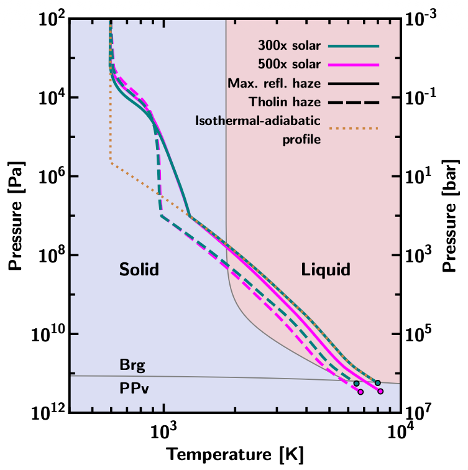
phase diagram for a common rocky material

A phase diagram for a common rocky material MgSiO3. The various lines show different model pressure–temperature profiles for the sub-Neptune GJ 1214b, while the circles indicate the location of the atmosphere/surface boundary. All circles fall into the “solid” part of the phase diagram, indicating that GJ 1214b likely has a solid surface. [Breza et al. 2025]

Somewhat surprisingly, the team found that about a third of the models they simulated had solid, not magma, surfaces. They found there were two distinct ways to solidify the magma and create a firm shell. First and most intuitively, if the surface temperature falls low enough, the magma will simply freeze. Second and more intriguingly, they found that a planet can also suppress a magma ocean if its atmosphere is heavy enough to drive up the surface pressure beyond the solid–liquid threshold.

This latter result is particularly insightful in light of recent JWST observations that suggest many sub-Neptunes have heavy atmospheres. These new models suggest that these worlds might have solid surfaces, and that models attempting to explain their compositions should be tweaked to account for this finding. In these early days where astronomers are still puzzling out the most basic properties of these strange worlds, research like this demonstrates the power of using advanced theoretical modeling to help interpret our cutting-edge observations.

Citation

“Not All Sub-Neptune Exoplanets Have Magma Oceans,” Bodie Breza et al 2025 ApJL 993 L46. doi:10.3847/2041-8213/ae0c07

The post Standing on a Sub-Neptune appeared first on AAS Nova.
A Black Hole Family Tree

31 October 2025 at 16:20

A rendering of two dark spheres surrounded by bright, misaligned disks drawing near to one another.

Black holes can have messy family histories, and a recent massive merger challenged astronomers to sort out just how many generations of black holes were involved in the event. Recent research, however, may have untangled the lineages of the two progenitors.

A Massive Collision

Earlier this year, the Laser Interferometer Gravitational-Wave Observatory (LIGO) detected the ripples in spacetime caused by the merger of two black holes somewhere in the distant universe. Though these detections have become increasingly common, this one in particular stood out among the more than 200 reported over the last decade. Named GW231123, this event must have caused more of a splash than a ripple since the two black holes that slammed together were unusually massive; both likely weighed more than 100 times the mass of the Sun. Not only that, each was also spinning unusually rapidly prior to the collision.

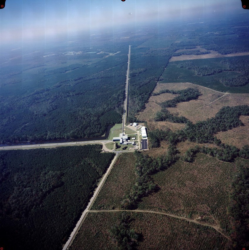
A photograph of two perpendicular straight lines that cut through a forest and meet at a complex of buildings in a clearing.

LIGO Livingston, one of the two LIGO detectors. [Caltech/MIT/LIGO Lab]

According to theory, black holes this large are not supposed to form on their own. When massive stars die, they can collapse into a black hole; but, when really massive stars die, the collapse is so violent that no material is left over to form the black hole. So, when researchers first measured the masses of the black holes involved in GW231123, they knew that the black holes involved couldn’t have formed directly from collapsed stars. Instead, they were likely second-generation black holes, meaning that they themselves formed from previous black hole–black hole mergers.

Merger Mystery

This result was celebrated as evidence of so-called “hierarchical formation,” in which black holes formed in dense environments swarm throughout their star clusters, merging with other black holes they encounter and growing ever larger.

However, there were a couple of complications with this picture. For one, theory predicts that it is challenging to form such rapidly spinning black holes from randomly oriented progenitors, since usually the spins wash out and leave the remnant rotating slowly. For another, the merging process tends to give the final black hole a “kick” that sends it flying rapidly away from the site of the impact, occasionally fast enough to leave the star cluster altogether, meaning second-generation black holes might not be able to merge into subsequent generations.

A multi-panel cartoon showing black holes merging through various combinations of 1st, 2nd, and 3rd generation black holes.

A schematic of various potential black hole family trees. The binary-star origin scenario is shown in the green box. Click to enlarge. [Stegmann et al. 2025]

Born as a Pair

New research led by Jakob Stegmann, Max Planck Institute for Astrophysics, suggests a way around each of these problems. In the team’s model, the two black holes involved in the GW231123 merger didn’t form from isolated black holes in a cluster, but rather from binary stars embedded within that cluster. In this picture, two massive stars were born bound together, orbiting one another within a larger cluster of stars. Crucially for this scenario, the massive primordial stars have aligned spins — an expected outcome of massive binary star evolution.

After both stars in the binary collapsed into black holes, these black holes merged to form a rapidly spinning second-generation black hole. This second-generation black hole eventually encountered another black hole within the cluster and merged to produce the ripples in spacetime we observed as GW231123.

Since black holes born within binary systems are expected to have smaller kicks and faster spins, this scenario neatly explains the properties observed in GW231123. As LIGO keeps listening for more black hole mergers, hopefully similar events will provide more chances to untangle their complex family trees.

Citation

“Resolving Black Hole Family Issues Among the Massive Ancestors of Very High-Spin Gravitational-Wave Events like GW231123,” Jakob Stegmann et al 2025 ApJL 992 L226. doi:10.3847/2041-8213/ae0e5f

The post A Black Hole Family Tree appeared first on AAS Nova.
Planets Can Be Bells: The Aftermath of Major Mergers

24 October 2025 at 17:00

A rendering of two rocky worlds mid-collision, with debris exploding outwards.

What would happen to a gaseous exoplanet if it was struck by a protoplanet? Recent research suggests that it would ring like a bell, and that just maybe, we’d be able to observe this ringing back on Earth.

Heavy Metal Mystery

Previous studies have hinted that giant planets have more heavy elements in their cores than we’d expect if they had formed from the exact same stew of gas and dust as their host stars. How exactly they end up with these enriched compositions is something of a mystery, though. Astronomers have proposed two potential theories: one somewhat dull, and one that involves dramatic collisions between the massive protoplanets.

In the first case, perhaps growing giant planets clear out the gas along their orbits, then steadily and quietly accrete the dust that spills over into the gaps. In the latter case, theorists have conjured a model in which growing gas giant planets repeatedly collide and merge with large and somewhat rocky protoplanets. Both of these mechanisms would produce the enhanced heavy element contents observed today, so how can we tell these two paths apart? Recent work by a team led by J.J. Zanazzi (University of California, Berkeley) proposes one such test.

Four spheres each showing a different oscillation mode, colored red and blue according to the change in temperature.

An illustration of the different oscillation modes within a gas giant after it’s struck by a protoplanet. [Zanazzi et al. 2025]

Ringing Planets

Through mathematical derivations, the researchers demonstrate that if a gas giant were to collide with a protoplanet, the impact would cause the planet’s surface to physically oscillate inwards and outwards, and for its surface temperature to vary. In other words, the planet would “ring” like a bell struck with a hammer, and as it physically convulses in the aftermath of the merger it would grow brighter and fainter in a repeating, periodic pattern. In principle, if the ringing lasts for long enough and the oscillations in brightness were large enough, observers back on Earth could record the amplitude and period of the changes and back out some constraints on what had happened and when.

An image of a bright disk, edge on, a coronograph mask blocking out the star, and a bright dot near the center of the mask.

An image of Beta Pictoris, including the young gas giant Beta Pictoris b and the surrounding debris disk. Click to enlarge. [ESO/A.-M. Lagrange et al.; CC BY 4.0]

Excitingly, the researchers demonstrate that not only would the oscillations last for millions of years, they would also be bright enough for JWST to detect for one specific planet named Beta Pictoris b. Should this world have undergone a merger in the last 18 million years, just a few hours of observations with JWST’s Near-Infrared Camera would reveal 45-minute pulsations in which the planet’s brightness changes by about 1%. Since the planet is too far away from its host star for these oscillations to be caused by any gravitational interactions, detecting any periodic signal would be a slam-dunk for the major merger theory.

Beta Pictoris b is a young planet in a system that’s still forming, and it orbits its host star on an eccentric path that takes it through dense regions of the disk. Hopefully, future observations will test whether this treacherous path produced any massive collisions in the relatively recent past. Until then, though, we can all enjoy charming visions of massive planets colliding with one another and ringing through the night.

Citation

“Seismic Oscillations Excited by Giant Impacts in Directly Imaged Giant Planets,” J. J. Zanazzi et al 2025 ApJ 993 3. doi:10.3847/1538-4357/ae04ec

The post Planets Can Be Bells: The Aftermath of Major Mergers appeared first on AAS Nova.
A Strange Brown Dwarf Gets Stranger

17 October 2025 at 17:00

A glowing orange sphere set against a background image of the Milky Way's disk of stars.

Isolated brown dwarfs are some of the rarest and hardest to study objects in our stellar neighborhood. Recently, astronomers revealed that one of the most famous isolated brown dwarfs, W1935, is not actually one brown dwarf but two.

Challenging but Fascinating

Astronomers know of only 50 free-floating brown dwarfs within the nearest 200 light-years or so, and even the ones we know about are poorly understood. Since brown dwarfs are frigid compared to their stellar cousins, they consequently shine much less brightly and at longer wavelengths of light. Even taking a picture of these ~500K objects requires long stares with specialized telescopes, and these facilities already have their schedules full supporting a wide range of other areas of research from distant galaxies to exploding supernovae.

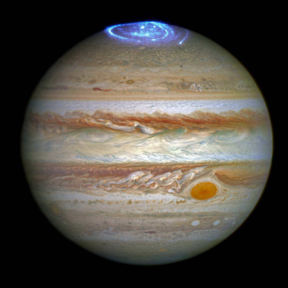
A color photograph of Jupiter showing its red bands, great red spot, and a bright spiraling blue aurora near the north pole.

An image of Jupiter and its prominent aurora taken with the Hubble Space Telescope. [NASA, ESA, and J. Nichols (University of Leicester); Acknowledgment: A. Simon (NASA/GSFC) and the OPAL team]

So, when an in-demand telescope like JWST spends time on brown dwarf science, each byte of data it sends back is both precious and likely to contain a new discovery. This has already happened several times: back in 2023, research published in the AAS journals (and summarized on AAS Nova) described JWST’s discovery of the first-ever Y+Y binary system, and in 2024, astronomers at the 243rd meeting of the AAS presented the first detection of methane emission on a brown dwarf — a sign of auroral activity.

Recently, JWST continued its pattern of discovery: the telescope took another look at the brown dwarf W1935, where methane emission was detected for the first time, and again found something surprising.

A New Binary

When JWST first took a look at this brown dwarf, it used its Near Infrared Spectrograph (NIRSpec) to record a spectrum of the object. These data revealed a large spike near 3 microns that perfectly lined up with methane emission from an aurora, similar to what we observe on Jupiter in the solar system. This was a thrilling find, since it hinted at an exciting possibility: Jupiter’s aurora is powered by its nearby moon Io, so the researchers cautiously wondered if W1935’s aurora could be evidence of a companion satellite as well.

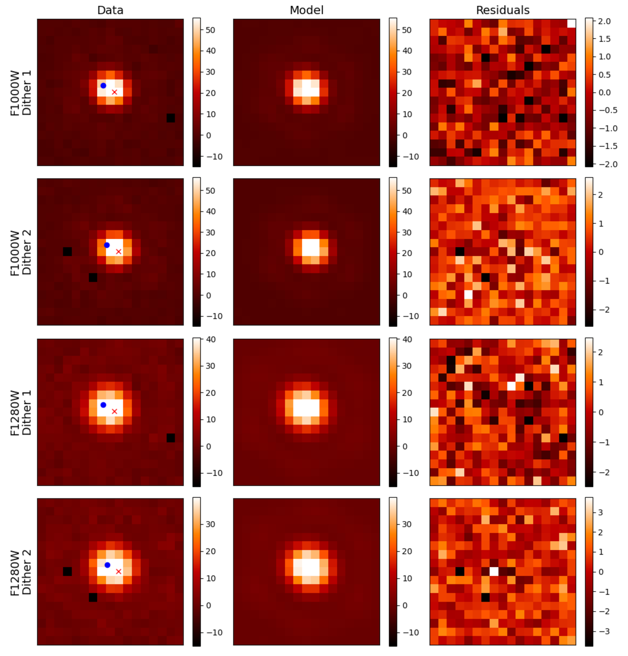
A multi-panel figure with noisy (real) images in the left column, smooth models in the middle column, and pixelated residuals in the rightmost column. The models are in good agreement with the data.

Images of W1935 taken with MIRI (left column), the author’s model for those images (center column), and the residuals (right column). The model includes two nearby point sources that are so close together they appear as one slightly elongated source. Click to enlarge. [De Furio et al. 2025]

Soon after these observations, JWST once again turned to W1935, but this time used its Mid-Infrared Instrument (MIRI) to take images of the object at long wavelengths. A team of researchers led by Matthew de Furio, University of Texas at Austin, recently analyzed these images and noticed something interesting: W1935 isn’t just one brown dwarf, but rather two roughly equal-mass brown dwarfs packed close together on 16–28 year orbits.

Doubly Interesting

This makes W1935 just the second-ever known Y+Y dwarf binary and cements its status as one of the most interesting brown dwarf systems discovered to date. So far, it’s not clear which object is responsible for the auroral signal since the objects are so close together that their images blur together without careful modeling and image processing.

De Furio’s team pointed out that JWST has yet another instrument that could prove useful here: its Integral Field Unit spectrometer within NIRSpec. Should JWST revisit this fascinating system, it could study the aurora’s variability over time, pin it to one specific object within the binary, and hopefully shed some light on whether any moons play a role in the methane emission. Given all we have learned each time JWST has turned to these strange worlds, we can only hope that it will do so again soon.

Citation

“Discovery of the Second Y+Y Dwarf Binary System: CWISEP J193518.59-154620.3,” Matthew De Furio et al 2025 ApJL 990 L63. doi:10.3847/2041-8213/adfee1

The post A Strange Brown Dwarf Gets Stranger appeared first on AAS Nova.
Researchers Spot a Rare Glowing, Growing Planet

8 October 2025 at 17:00

WISPIT 2b

Have you ever eaten a meal so quickly that you started to glow? Although this behavior likely isn’t relatable for most humans, astronomers are beginning to find more and more baby planets doing just that.

Planetary Glow Up

Planets are, famously, quite large. But astronomers know that they don’t start out that way, and that instead, stars and planetary systems start as wispy collections of dust and gas. This raw material eventually compresses itself into stars and planets and life capable of contemplating such things, but how exactly that happens is not perfectly understood.

A colored-pencil drawing of gas flowing around a planet, with arrows noting the direction of the flow at various points.

A schematic of some of the processes involved during giant planet formation. Click to enlarge. [Batygin 2018]

Astronomers have the broad contours sketched out at least. Protoplanets destined to become gas giants like Jupiter and Saturn start by gobbling up all the material around them and eventually clear out gaps in the disks in which they are born. What little material flows into these gaps gets sucked onto the planet in a process called accretion, though exactly where this material lands and how gravity and magnetic fields interact is up for debate.

A number of different mechanisms predict that during this process, the protoplanet should emit light at a certain frequency associated with electrons jumping between energy levels in hydrogen atoms — what astronomers call Hα emission. In other words, they should glow at that specific wavelength only when they are accreting, though how strongly and consistently will depend on exactly what is happening around the planet.

These ideas existed only on paper until 2019, when a team first observed two glowing, growing planets around the star PDS 70. Recently, however, a powerful new instrument has begun collecting data, and astronomers just announced it has found another similar protoplanet: WISPIT-2b.

A New Discovery

A team of researchers led by Laird Close (University of Arizona) announced the discovery of this new world after analyzing images taken with the powerful new MagAO-X instrument on one of the 6.5-meter Magellan telescopes in Chile. The team outfitted the camera with a narrow filter that only admitted the Hα emission associated with accretion, then collected thousands of images over about two hours in April 2025. After stacking and post-processing their data, a faint dot jumped out beside the central star, right in the gap between two bright rings in the star’s disk.

A bright dot beside fainter rings of material.

A follow-up image of WISPIT-2b taken with a broader filter. [Laird et al. 2025]

This protoplanet, which the authors name WISPIT-2b in honor of their Wide Separation Planets in Time (WISPIT) survey, is likely about five times the mass of Jupiter and only 5 million years old, making it a baby on astronomical timescales. Based on how strongly it’s glowing, the team estimates that it’s accreting the equivalent of about 100 times the mass of Phobos, Mars’s largest moon, each year. This process won’t continue forever, as eventually the remains of the star’s disk will disperse and the planet will have to go hungry.

This remarkable find is only the third protoplanet unambiguously found to be embedded within a disk, and the first to be found in the gap between rings in a disk. With MagAO-X collecting data and the WISPIT survey underway, we’re likely in store for many other discoveries in the coming years. With enough observations and examples of these growing worlds, astronomers will fill in their models of how exactly giant planets as we know them are formed.

Citation

“Wide Separation Planets in Time (WISPIT): Discovery of a Gap Hα Protoplanet WISPIT 2b with MagAO-X,” Laird M. Close et al 2025 ApJL 990 L9. doi:10.3847/2041-8213/adf7a5

The post Researchers Spot a Rare Glowing, Growing Planet appeared first on AAS Nova.
Kicking Neutron Stars from the Nest

24 September 2025 at 17:00

A blue/white star with lines representing magnetic fields sprouting from the poles against a black background.

Neutron stars don’t stick around for long after they’re born. Recent research has now uncovered just how fast they flee.

They Grow Up So Fast

Human beings require many years of care and support from their parents before they’re able to venture forth into the world. This is an embarrassingly long process compared to the standard for animals like deer and horses, whose offspring are ready to walk mere minutes after birth. However, baby neutron stars, some of the densest objects in the known universe, put all life on Earth to shame with their immediate self-reliance: after a fiery birth from a supernova explosion, these stars flee the site of their creation at hundreds of kilometers per second.

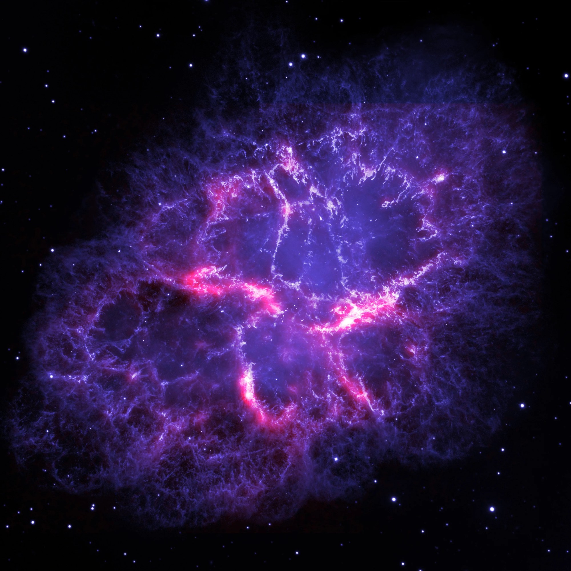
Crab Nebula supernova remnant

Hubble Space Telescope and Herschel Space Observatory image of the Crab Nebula, which is the remnant of a supernova explosion. [ESA/Herschel/PACS/MESS Key Programme Supernova Remnant Team; NASA, ESA and Allison Loll/Jeff Hester (Arizona State University)]

These “natal kicks,” as they’re called in research literature and in recent work by Paul Disberg and Ilya Mandel (Monash University and OzGrav) are a natural consequence of neutron star formation. When a massive star burns through the last of its fuel and surrenders to its own gravity, it collapses inward and compresses its core into a neutron star before rebounding in an explosion. This collapse is never perfectly symmetric, however, and the slight imbalance gives the resulting neutron star a shove.

By measuring the characteristic speeds of these “kicks,” astronomers can deduce how asymmetric the preceding collapse must have been, along with other information about the earliest moments of the supernova. Though measuring the speed of something so small from the other side of the galaxy is no easy task, Disberg and Mandel’s recent publication in The Astrophysical Journal Letters takes on the challenge.

Quantifying the Kicks

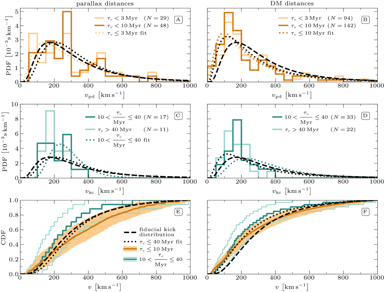
The pair first began by examining measurements of neutron stars known to be less than 10 million years old, which is extremely young in an astronomical context. Since these objects haven’t had time to be slowed down or altered from their course by passing stars or the galactic tide, their present-day speeds should be the same as their natal kicks. The researchers found that while every neutron star had its own unique kick velocity, the distribution of all the velocities followed a log-normal pattern with a peak near 150–200 km/s.

Measured kick velocities and fit distributions

Measured kick velocities (histograms) and fit distributions (curves) for different subsamples. Click to enlarge. [Disberg & Mandel 2025]

Next, Disberg and Mandel examined the distribution of velocities from older neutron stars. These, which had to be measured via a different method, turned out to be very similar to the distribution assigned to the younger stars. Finally, they re-examined previous studies that attempted their own models of the kick distribution. Though several of these studies conflicted with one another, the team found that these discrepancies could be explained by different sample sizes and mistaken statistical interpretations. On the whole, the team’s distribution fit all the available data well and the most succinctly of any alternative framework.

Going forward, other astronomers focused on modeling supernovae, orbits within the galaxy, and binary-star evolution can use this distribution either to sanity check their models or as inputs to other simulations. Through slow accumulation of studies like this, each with its own quantified measurement of some property in the galaxy, we come to understand our universe more fully and unlock our ability to make ever more models and predictions.

Citation

“The Kick Velocity Distribution of Isolated Neutron Stars,” Paul Disberg and Ilya Mandel 2025 ApJL 989 L8. doi:10.3847/2041-8213/adf286

The post Kicking Neutron Stars from the Nest appeared first on AAS Nova.
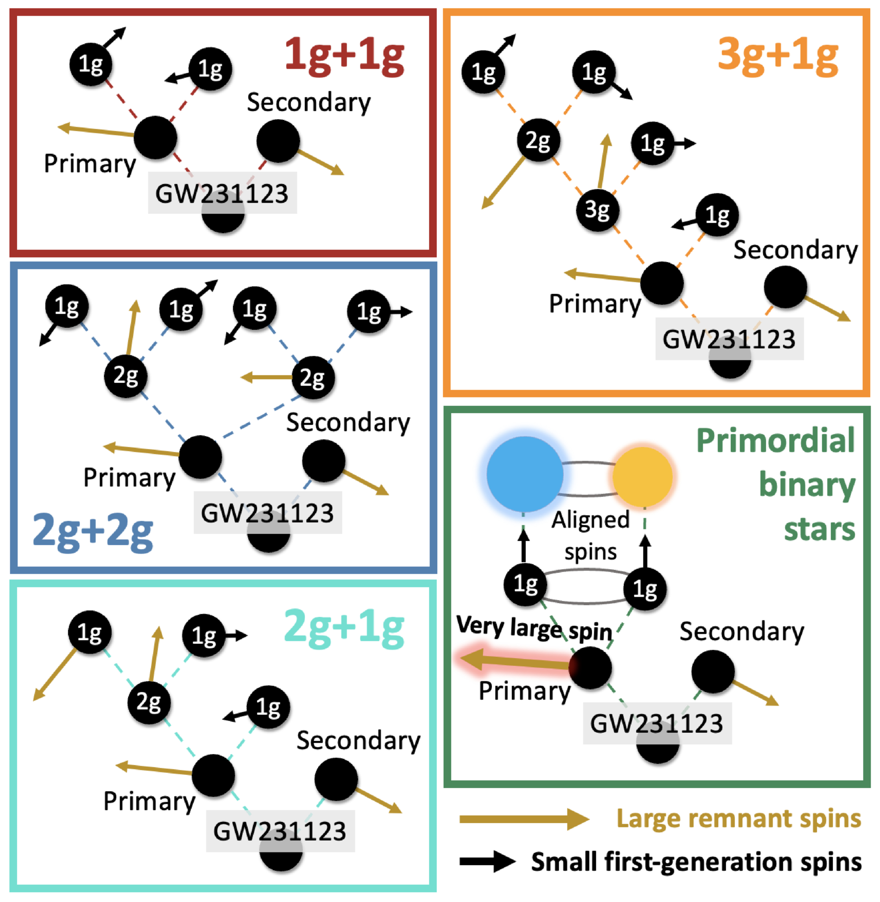
Cluster Before Stack: A New Algorithm for Pulsar Timing

19 September 2025 at 17:00

A photograph of a large radio dish taken during the day from above.

To measure properties of a pulsar accurately, astronomers have to stack many individual observations together to boost the signal above the noise. But what if there was a more clever, more effective way to add observations than simple stacking?

Weak Cosmic Lighthouses

Pulsars, or rapidly spinning neutron stars that emit narrow cones of radio waves, are often referred to as the galaxy’s lighthouses. Just like a sailor looking to shore might see a periodic flash when a lighthouse’s beacon sweeps over their ship, so too would radio telescopes aimed at a pulsar detect a “pulse” when its beam sweeps across Earth. However, although this comparison to lighthouses is a powerful analogy, it starts to break down when considering the speed and strength of these flashes.

A time series showing a Gaussian-like spike.

An example of one noisy individual pulse. Click to enlarge. [Sosa Fiscella et al. 2025]

While lighthouses may take several seconds to rotate their lens and lamp once around, pulsars do the same in just a few milliseconds. What’s more, while lighthouses are designed to be bright enough that sailors can notice every individual flash, pulsars are comparatively dim. To confidently measure the “pulse profile,” or how a pulsar’s radio intensity changes as a function of its rotation phase, astronomers need to stack those hundreds of thousands of pulses together into one artificial super-bright pulse. Only then can they measure the quantities they care about, like the precise spin period and average pulse arrival time.

This practice rests of the subtle assertion that every individual pulse is just a noisy variation of the same unchanging pulse profile. But is that safe to assume? And can we improve the precision of our measurements by doing something more complex than simple stacking? These are the questions recently tackled by a team of astronomers led by Sofia V. Sosa Fiscella (Rochester Institute of Technology) in research published in The Astrophysical Journal.

Squeezing the Data

The researchers focused on one particularly bright source named PSR J2145−0750 that was observed by the Green Bank Telescope for two hours in 2017. This pulsar is so bright that it’s possible to measure quantities like the pulse width, height, center, and total energy of individual pulses, not just the final stack. The team did just that for each of the more than 200,000 pulses in their dataset and assigned each one a vector of four numbers. When they next sorted the pulses into distinct groups, they found that there were indeed correlations among these variables: for example, pulses with higher maximum heights tended to arrive earlier and be narrower than the overall average.

A 3D plot across different measured pulse characteristics where each point is colored according to its cluster.

A visual representation of the different pulse clusters. Each point corresponds to one pulse. Click to enlarge. [Sosa Fiscella et al. 2025]

To take advantage of this structure, they created a stacked pulse profile for each cluster, measured the center in each of them, then averaged all the cluster-specific times together into a final answer. While the standard method of stacking all of the data into one pulse profile resulted in a timing precision of 0.066 microsecond, this new method shrank the uncertainty to 0.057 microsecond, a meaningful improvement.

Though the team cautions that this new method will likely only be relevant for the pulsars for which we can measure individual pulses, they also point out that as better telescopes come online, we’ll be able to do that for more pulsars. In the meantime, astronomers can take comfort in the fact that as our technological abilities improve, so do our abilities to squeeze as much from our data as possible.

Citation

“Improving Pulsar Timing Precision with Single Pulse Fluence Clustering,” Sofia V. Sosa Fiscella et al 2025 ApJ 984 111. doi:10.3847/1538-4357/adc1c2

The post Cluster Before Stack: A New Algorithm for Pulsar Timing appeared first on AAS Nova.
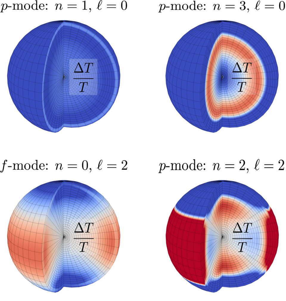
Scars from a Black Hole

10 September 2025 at 17:00

A spiral of bright material circling a black core.

Simulations suggest that there should be a million stars in our galaxy that once wandered so close to a supermassive black hole that they were nearly destroyed. What are the long-term effects of this encounter, and could astronomers observe the scars of these near-death experiences?

Moths to a Flame

center of the Milky Way

This infrared and X-ray image of the Milky Way’s center shows a swirl of hot gas surrounding Sagittarius A*, our galaxy’s central supermassive black hole. [NASA, ESA, SSC, CXC, STScI]

The center of our galaxy is a dangerous place to be a star. Like mosquitoes drawn to a light, millions of stars swarm around the supermassive black hole named Sagittarius A*, packing themselves in tight and kicking one another onto wild, eccentric, and ever-changing orbits. Every 100,000 years or so, one of these stars gets an unlucky push and finally gives in to the black hole’s irresistible pull. A nudge from a neighbor will send it hurtling beyond the point of safety, and in one intense flyby, it’ll be ripped apart by Sagittarius A*’s immense gravitational field.

Simulations suggest that most of the time, these hapless stars are not completely destroyed by their close encounters with the black hole. In principle, then, there should be about a million “survivor” stars wandering near the center of our galaxy. But, what would these survivors look like? And with careful measurements, could we tell them apart from their regular, unscathed counterparts?

Simulating a Star’s Worst Day

Recently, a team of astronomers led by Rewa Clark Bush (University of California Santa Cruz, Cabrillo College, Wesleyan University) tackled this question. First, the team needed to simulate a terrible day for a hypothetical star: the day it passes closest to the black hole. To compute what happens to the star in those intense couple of hours, they used an open-source hydrodynamic code called FLASH to track the state of the star in granular detail.

An 8-panel figure showing complex, asymmetric patterns of gas around a dense core.

Temperatures (top row) and diffusion timescales (bottom row) of four stars soon after their closest approach to the black hole. Click to enlarge. [Bush et al. 2025]

Then, once the star (or what was left of it) managed to flee back to safety, the team froze the simulations and took stock. They found that depending on the initial size of the star and the distance of its closest approach, the black hole stripped away anywhere from a few percent to almost two thirds of the star’s mass. The researchers then fed the stars into another code called MESA to simulate how the disturbed stars would settle into a new equilibrium and evolve over billions of years.

Back on Track

Plot comparing disturbed and undisturbed stars

Comparison of the original undisturbed stars (filled circles), the stars after a black hole encounter (open symbols), and other stars with different initial masses (black points). Click to enlarge. [Bush et al. 2025].

The team found that although these unlucky stars likely glow tens to hundreds of times brighter than usual after their flyby, this period of enhanced brightness lasts less than 100,000 years. For our galaxy, this translates to 1–10 stars currently in the galactic center that have been brightened by an encounter with a supermassive black hole.

Eventually, though, these stars pretty much return to a new normal. Though these stars would have had slightly different colors and luminosities had they not encountered the black hole, they end up looking similar to undisturbed stars with the same final mass.

Although detailed spectroscopic measurements of these remnants might reveal a strange composition thanks to all the stirring that happened during the flyby, it’d be hard to tell anything happened to these stars otherwise. Ultimately, life goes on, even for stars that were nearly destroyed by the most massive creature in the galaxy.

Citation

“Black Hole Survival Guide: Searching for Stars in the Galactic Center that Endure Partial Tidal Disruption,” Rewa Clark Bush et al 2025 ApJL 990 L7. doi:10.3847/2041-8213/adefde

The post Scars from a Black Hole appeared first on AAS Nova.
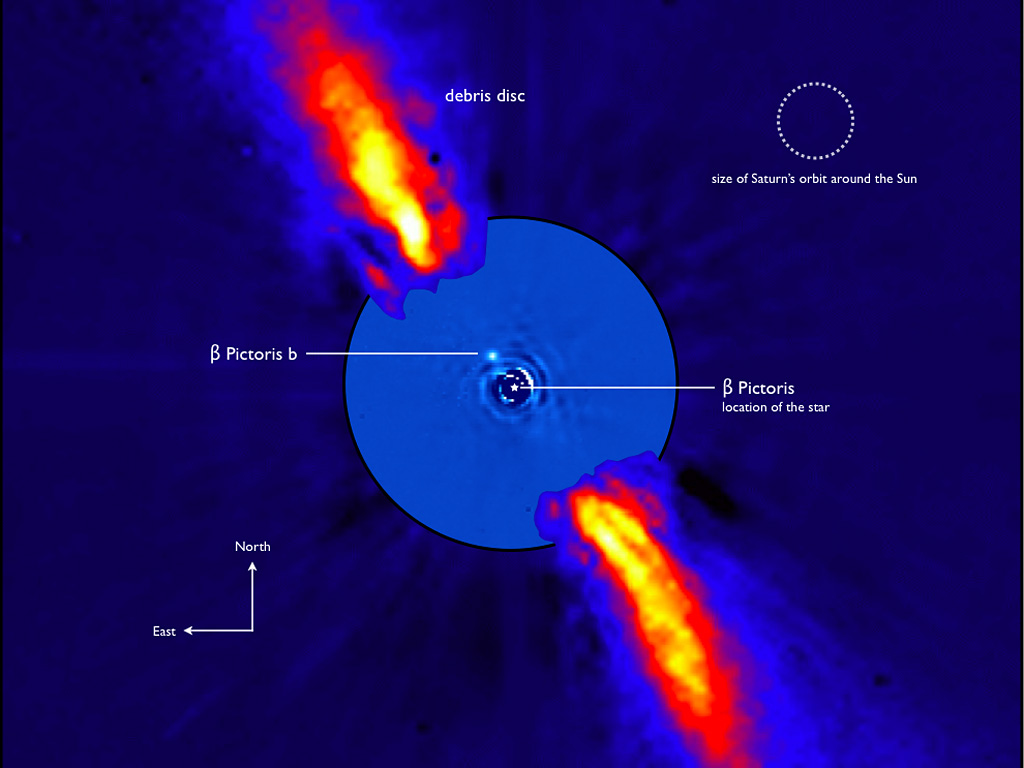
❌