❌

Normal view

Primordial Planetesimals from the Guts of Population III Stars

2 September 2026 at 21:45

Protoplanetary Disk

While previous investigations of planet formation across the universe’s history suggest that planets trickled into the picture, a recent study has found that primordial planetesimals could have formed much earlier from the insides of the first stars in the universe.

First Stars, First Planets?

When the first stars flickered on, the universe was filled with pristine gas, containing only hydrogen, helium, and a little lithium. This gas, though great at making massive stars known as Population III (Pop III) stars, was not yet enriched with the heavy elements necessary for planet formation and, of course, life. Past studies have suggested that planet formation in the universe was gradual, taking several billion years to peak after billions of stars created and spilled the needed metals into the universe. However, local pockets of enriched gas from Pop III stars could have created the right conditions for planet formation earlier in the universe’s history.

Pop III stars burned bright and fast, exploding violently in pair-instability supernovae that completely shredded the progenitor, ejecting over 100 solar masses of metals into their previously pristine surroundings. Cosmological simulations suggest that oxygen from these supernovae could have produced significant water fractions within the dense cores of the supernova remnant. This may have set the stage for planet formation in water-rich disks around subsequent generations of stars as early as 150–200 million years after the Big Bang — does numerical modeling support this planet formation hypothesis?

Protoplanetary disk growth

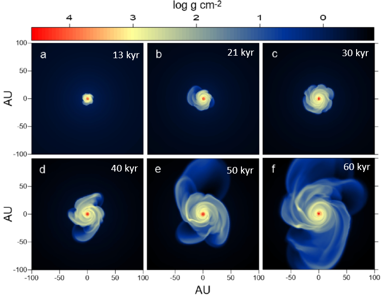
Simulation snapshots showing the formation and evolution of the protoplanetary disk for 13, 21, 30, 40, 50, and 60 thousands of years after protostellar birth. Click to enlarge. [Modified from Vorobyov et al 2026]

Primordial Planetesimals in Simulated Water-Rich Disks

To test if these water-rich dense cores within Pop III supernova remnants could form planetesimals, the building blocks of terrestrial planets, Eduard I. Vorobyov (University of Innsbruck; Southern Federal University) and collaborators performed numerical simulations tracing the collapse of one such gas core into a protoplanetary disk around a protostar. The simulations begin from the gravitational collapse of a 1-solar-mass gas cloud core, with a protostar emerging 24 thousand years after the initial cloud collapse. As the protostar’s gravity pulled in material from its surroundings, a rotating disk formed around the growing star.

Protoplanetary disk evolution and planetesimal growth

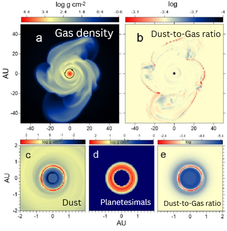
Simulation snapshot 40 thousand years after the formation of the protostar showing the gas, dust, and planetesimal surface densities and the dust-to-gas ratio. Click to enlarge. [Modified from Vorobyov et al 2026]

Tracking the gas and dust evolution in the disk, the authors found that several Earth masses of planetesimals formed within 0.5–1.0 au of the 0.4-solar-mass protostar. While the simulations did not trace the disk all the way to planet formation (this requires complex multi-body modeling and lots of computing power), enough planetesimals formed to create a Mars- or Earth-mass planet in the future. Luckily, unlike their live-fast and die-young predecessors, low-mass stars born from Pop III supernova remnants would still be burning hydrogen in their cores today, and ancient metal-poor stars in the Milky Way’s halo may be home to the universe’s first planets that could be detected in future exoplanet surveys. This study showed, for the first time, that water-rich protoplanetary disks with planetesimals could pop up billions of years earlier than previously thought, changing our understanding of planet formation in the universe.

Citation

“Planet Formation at Cosmic Dawn: Planetesimals in H2O-rich Disks around Low-mass Stars,” Eduard I. Vorobyov et al 2026 ApJL 1007 L51. doi:10.3847/2041-8213/ae907c

The post Primordial Planetesimals from the Guts of Population III Stars appeared first on AAS Nova.

U.S. Department of Defense Initiative Funds AI Scientists to Help Predict the Future on the Battlefield

19 August 2026 at 14:03

The United States Department of Defense has funded an effort by SUNY Polytechnic Institute scientists to use artificial intelligence to evaluate complex defense scenarios before they unfold, including real-time predictive analysis of multiple potential scenarios in a concerted effort to predict the future on the battlefield.

DoD and SUNY Poly officials said the ‘landmark’ $61.8 million award, which will directly support the U.S. Army Transformation Decision Analysis Center (TDAC), will use advanced, data-driven analytical tools to offer the U.S. Army an unprecedented tactical advantage, improving preparedness and reducing uncertainty in high-stakes decision-making battlefield environments

“The initiative aims to provide commanders with a decisive strategic advantage in an increasingly volatile global landscape by integrating high-velocity AI into the Army’s core decision-making frameworks,” a statement announcing the new award explained.

Using AI to Predict the Future Helps Army “Respond to Evolving Threats”

The first phase of the effort to use AI to predict the future will focus on synchronizing military operations in several critical domains, including land, air, space, and cyberspace. The team, which includes researchers from the University of South Florida and the University System of Maryland, said this phase will emphasize integrating generative AI, foundation models, and advanced inference systems to “simulate complex operational scenarios and provide predictive insights.”

“These tools will enable the Army to better assess risks, evaluate strategies, and respond to evolving threats in both competitive and crisis environments,” they explain.

As the SUNY Poly-led team moves into future phases, it will also explore several “advanced” capabilities not covered in the initial phase. For example, the team will evaluate synthetic data generation and anomaly detection. The announcement said the team also plans to explore large language models (LLMs) and time-series foundation models to “enhance situational awareness.”

Other areas of focus include AI system security and reliability, including the ability to operate in “adversarial and resource-constrained environments.” Critically, this effort also includes ensuring robust AI performance “even under cyber threats or disrupted conditions.”

Evaluating Complex Scenarios Before They Unfold

One of the more intriguing components of the new award involves simulating battlefield environments to predict the future. Specifically, the team said it hopes to use battlefield simulations to enable “spatial reasoning through the integration of generative AI and active inference models.”

“These innovations will allow military planners to evaluate complex scenarios before they unfold, improving preparedness and reducing uncertainty in high-stakes decision-making,” the statement explains, adding that the effort will “contribute to the Army’s broader modernization strategy, supporting the development of next-generation analytical tools that inform readiness, capability development, and operational planning.”

Dr. Michael Carpenter, Vice President for Research at SUNY Poly, said the work represents a major step forward for the integration of AI and machine learning to “support resilient and adaptive decision-making for the Army.”

“Our team is developing sophisticated models that can synthesize vast amounts of data, generate realistic scenarios, and provide actionable intelligence,” Dr. Carpenter explained. “These capabilities will be critical in helping the Army anticipate challenges and maintain a strategic edge.”

After noting their honor at receiving the award, SUNY Poly President Dr. Winston Soboyejo said the DoD’s confidence in their program “reflects SUNY Poly’s research excellence and our commitment to solving the nation’s most complex security challenges.”

“By working closely with our partners, we will deliver transformative technologies that ensure the Army remains agile, informed, and ready for any multi-domain conflict,” Dr. Soboyejo concluded, adding that “we are proud to contribute to technologies that advance science and engineering, and strengthen national security and global stability.”

Christopher Plain is a Science Fiction and Fantasy novelist and has spent the last six years as Associate News Editor and Head Science Writer at The Debrief. Follow and connect with him on X, learn about his books at plainfiction.com, or email him at christopher@thedebrief.org

The “Rhythm” of the Interstellar Medium

28 July 2026 at 17:00

Messier 17

Editor’s Note: Astrobites is a graduate-student-run organization that digests astrophysical literature for undergraduate students. As part of the partnership between the AAS and astrobites, we occasionally repost astrobites content here at AAS Nova. We hope you enjoy this post from astrobites; the original can be viewed at astrobites.org.

Title: The Rhythm of the ISM: Tracing the Timescales of Gas Evolution and Star Formation Across Galactic Environments
Authors: Zuzanna Kocjan and Vadim A. Semenov
First Author’s Institution: University of Maryland
Status: Published in ApJ

The Connection Between Gas and Star Formation in Galaxies

Stars are born in the interstellar medium (ISM) when cold, dense clouds of gas become unstable and collapse under gravity. Despite their plentiful reservoirs of gas, galaxies convert only a small fraction of this material into stars, making star formation a surprisingly inefficient process. A key factor behind this inefficiency is stellar feedback: radiation, stellar winds, and supernova explosions from young stars can inject energy and momentum into the surrounding gas, heating, stirring, and dispersing it. In this way, stellar feedback shapes future star formation across scales ranging from individual regions in the ISM to whole galaxies.

An important tool astronomers use to study star formation is the Kennicutt–Schmidt relation, which links the amount of gas in a galaxy to the rate at which stars form. More specifically, it relates the gas surface density, Σgas, to the star formation rate surface density, ΣSFR. (For more on this relation, see this Astrobites article on a classic research article.) However, this law is underpinned by a crucial ingredient: timescales. In particular, the pace of star formation depends both on how quickly galactic gas is cycled into star-forming material and on how rapidly those regions convert gas into stars once they form. Today’s article investigates the physical origin of star-formation scaling relations behind the Kennicutt–Schmidt law by building on a simple theoretical framework for the ISM.

Consider a Kettle of Boiling Water…

In a given region of a galaxy, the ISM consists of gas in either an actively star-forming state or an inert, non-star-forming state, depending on whether it is dense and unstable enough to collapse (as illustrated in Figure 1). The transition of non-star-forming gas into the star-forming state occurs on the supply timescale, τ+. Conversely, the dispersal of star-forming gas back into a non-star-forming state is characterized by the removal timescale, τ–. As a helpful analogy, the authors compare this process to water boiling in a kettle: the ISM is continuously “boiling,” with gas moving between active and inactive states. Meanwhile, the total gas reservoir gradually decreases, analogous to water slowly evaporating as the kettle boils. The gas depletion time, τ*, therefore represents the timescale over which the available gas would be exhausted by star formation.

Schematic of the gas cycling framework

Figure 1: Schematic of the gas cycling framework used in the authors’ theoretical model for how gas is converted into stars, which takes into account a supply, removal, and depletion timescale. [Adapted from Kocjan and Semenov 2026]

Building on this picture of gas cycling, the authors turn to simulated galaxies, where the motion and evolution of the gas can be followed directly. By tracking how gas flows through the ISM in the simulations, they derive the three characteristic timescales above — τ+, τ–, and τ* — that describe how gas is supplied to, removed from, and ultimately consumed by star formation. The goal is to connect the small-scale physics of the ISM to the large-scale star formation efficiencies and scaling relations observed across galaxies.

The Timescales of the Interstellar Medium

To explore how gas and star formation are connected across different galactic environments, the authors analyze three simulated systems: a dwarf galaxy, a Milky Way–like galaxy, and a gas-rich starburst galaxy, as shown in Figure 2. Despite spanning very different physical regimes, the galaxies exhibit remarkably similar trends in the fraction of gas actively forming stars as a function of Σgas​. This suggests that the amount of star-forming gas is governed primarily by local interstellar conditions, since regions with higher gas surface densities tend to contain denser, more strongly self-gravitating gas.

galaxy simulations and star-forming gas fraction

Figure 2: Using simulations (left to right) of an isolated intermediate-mass dwarf galaxy, Milky Way–like galaxy, and gas-rich galaxy, the authors measure the star-forming gas fraction versus the gas surface density (right). [Adapted from Kocjan and Semenov 2026]

To further understand this trend, this study then applies the authors’ theoretical framework to determine the timescales of ISM gas cycling on the scales of individual star-forming regions. These include the timescales for the formation, dispersal, and local depletion of star-forming gas as described above: τ+, τ−, and τ∗, which also exhibit strong correlations with the gas surface density (see Figure 3). Specifically, the timescale for supplying gas into the star-forming state is linked to the rate at which turbulence redistributes material through the galactic disk. The depletion timescale, over which star-forming gas is turned into stars, decreases at higher Σgas​, since denser regions more efficiently collapse and form stars. By contrast, the removal timescale is comparatively short, reflecting how quickly feedback and changes in local equilibrium can disrupt star-forming clouds. In this way, the “boiling kettle” framework is able to capture the major processes driving small-scale gas evolution.
Scaling relations between the supply, depletion, and removal times

Figure 3: Scaling relations between the supply (left), depletion (middle), and removal (right) times in kiloparsec-scale regions of the simulated galaxies (shown in different colors). Based on the measurements from the simulations, the authors introduce a parameterized model for the gas cycling framework, as defined in the equations. [Adapted from Kocjan and Semenov 2026]

The cycling of gas through different phases of the ISM offers a useful framework for understanding how galaxies form stars. In the relatively well-ordered systems studied here, this balance can be described in simple terms; however, it is likely to become more complex in extreme environments where additional physical processes — such as those operating in the early stages of galaxy formation — play a significant role. Even so, these results highlight how key galactic properties can emerge naturally from the interplay between galaxy-scale dynamics, ISM turbulence, and the state of star-forming gas.

Original astrobite edited by Jayde Willingham.

About the author, Shalini Kurinchi-Vendhan:

After studying astrophysics and literature at Caltech, I moved onto a Fulbright Fellowship in Heidelberg, Germany. I’m passionate about using computer simulations to explore supermassive black holes and galaxy evolution — but I also love poetry and traveling.

The post The “Rhythm” of the Interstellar Medium appeared first on AAS Nova.

Detached but Not Alone

26 June 2026 at 17:00

A rendering of a Jupiter-like planet floating in front of a galaxy.

Microlensing surveys have discovered plenty of regular exoplanets, but more surprisingly, they’ve also turned up many solo Neptunes with no star nearby. New research suggests that first impressions might be deceiving, however, and that at least some of these planets might not be so alone: they just have a complicated family history.

An Abundance of Exo-Neptunes

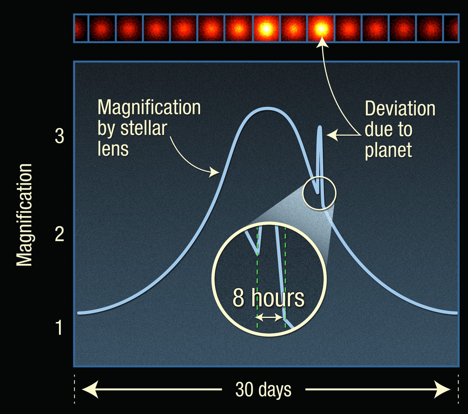
There are simply too many Neptune-like exoplanets in our galaxy. Or at least that’s the current feeling astronomers get from gravitational microlensing surveys, which look for exoplanets during short-lived magnification events caused by chance alignments between stars. These surveys have now found about a dozen so-called “free-floating” planets, and while this doesn’t sound like that many, running the numbers reveals that this tiny sample implies that there are about two free-floating Neptune-size planets for every star in the galaxy.

A schematic graph of a large pulse and a smaller narrower pulse superimposed on top.

An illustration of how exoplanets are found via microlensing. The broad first bump is caused by the host star magnifying the light from a background star; the narrow second bump is caused by the planet acting as a lens as well. “Free-floating” planets create only one bump. [Adapted from NASA, ESA, and A. Feild (STScI)]

The idea that there are more free-ranging Neptunes than stars is unsettling, and astronomers aren’t yet sure how this many planets ended up so isolated. It’s possible that these objects simply formed disconnected from any planetary system, but it’s unclear how something so small could collapse from the interstellar clouds that usually produce stellar-mass objects. It’s also possible that the planets formed around stars in the usual way, only to be later kicked out by some violent dynamical process — but this would either require too much time or too many giant planets capable of ejecting the lower-mass ones.

However, new research by Sam Hadden (Canadian Institute for Theoretical Astrophysics) and Yanqin Wu (University of Toronto) presents an alternative idea: what if at least some of these free-floating planets aren’t fully on their own, but instead remain estranged but weakly bound to their parent stars?

Simulated Scattering

Two celestial objects need to align nearly perfectly in order to create a microlensing pulse that we can detect. For an exoplanet orbiting a star, we should observe two of these pulses: one when the host star drifts in and out of alignment with a background star, and one when the nearby bound planet does the same. In the case of a free-floating planet, there’s only one pulse, and we therefore assume that there is no host star. Hadden and Wu noticed that since the alignment has to be so precise for microlensing to occur, it’s possible that a seemingly free-floating planet is simply widely separated from its host star, and the star managed to dodge the magnification effect. In other words, these planets might not be free floating at all, just on wide and eccentric orbits.

A two-panel plot showing how the semimajor axis and inclination of 5 planets evolve over time.

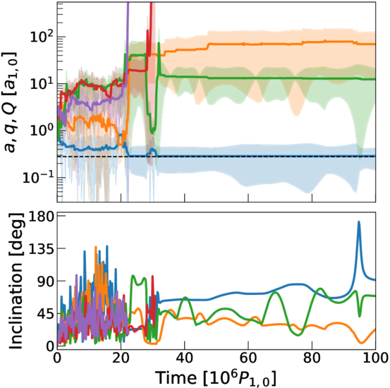
The orbital evolution of a five-planet system that undergoes planet–planet scattering. Each line represents one planet; note that in the end two are ejected, two end up on wide detached orbits, and the fifth ends up on a tightly bound inner orbit. Click to enlarge. [Hadden & Yu 2026]

The researchers decided to test whether it’s possible to create these kinds of orbits via a known dynamical process called planet–planet scattering. As the name implies, during this process, planets that begin on orderly orbits around their parent star undergo a dramatic rearrangement as they jostle each other around through gravitational interactions. The researchers created two types of simulations: one with a collection of equal-mass planets, and another in which one planet dominates over a brood of smaller ones. After setting up the systems, they let the “dynamical havoc” proceed for a few hundred million years, then surveyed the aftermath.

They found that both types of simulations readily created the “detached” objects needed to mimic free-floating planets. In fact, the most common outcome was for two or three planets to be bullied into far-out orbits by a planet that then plunges onto a tight inner orbit extremely close to the star.

Though the authors caution that this process likely doesn’t explain all of the free-floating planets observed to date, this is an exciting model that would dramatically lower our estimates of the number of Neptunes roaming alone between the stars.

Citation

“Free Floating or Merely Detached?,” Sam Hadden and Yanqin Wu 2026 ApJ 1000 70. doi:10.3847/1538-4357/ae6508

The post Detached but Not Alone appeared first on AAS Nova.

Human Impact Quadruples Coastal Sea-Level Extremes

16 June 2026 at 14:59

In a groundbreaking study published in Nature Climate Change, scientists have unveiled compelling evidence that human-driven sea-level rise has drastically intensified the frequency of extreme coastal flooding events since the dawn of the 20th century. This new research, led by Dangendorf and colleagues, synthesizes extensive tide-gauge data with historical climate model simulations, revealing that the incidence of once-rare 1-in-100-year coastal flooding events has surged approximately twelvefold on a global scale. The findings highlight an unsettling reality: anthropogenic radiative forcing has quadrupled the likelihood of such extremes, fundamentally reshaping the landscape of coastal hazard risk worldwide.

For decades, the debate around the extent to which human activities have contributed to sea-level rise and associated coastal flooding has been mired with uncertainties. Previous studies often grappled with limited observational records or lacked the comprehensive modeling necessary to isolate human influence from natural variability. The novel detection and attribution framework employed in this study marks a significant advancement by bridging long-term tide-gauge observations—some extending back over a century—with sophisticated simulations from the Coupled Model Intercomparison Project Phase 5 (CMIP5). This approach allowed the researchers to untangle complex interactions and discern the fingerprints of anthropogenic climate forcing with unprecedented clarity.

The critical driver identified by the team is relative sea-level rise, a multifaceted phenomenon encompassing both ocean surface height changes and vertical land movements relative to the coast. Since the 1960s, this relative sea-level rise has been overwhelmingly dominated by human-induced factors, principally the accumulation of greenhouse gases in the atmosphere that trap heat and accelerate melting of ice sheets and glaciers. As sea levels climb, coastal areas become increasingly susceptible to flooding from storm surges, high tides, and extreme weather events that were historically rare or even unheard of.

Statistically, this change translates into dramatic shifts in risk profiles: an event that would have been expected once every century historically now occurs on average every eight years globally. In some regions, the frequency increase is even more pronounced, reflecting the heterogeneous nature of sea-level rise and the role of localized factors, such as land subsidence or ocean currents. This amplification of coastal extremes poses grave implications for millions of people living in low-lying coastal zones, threatening infrastructure resilience, habitability, and economic stability.

Furthermore, while natural variability—cycles such as the El Niño Southern Oscillation or decadal ocean oscillations—continues to influence regional patterns of extreme sea-level frequency, the study finds this factor has become secondary along the majority of the world’s coastlines. The persistent upward trend linked to human-induced climate change overrides traditional weather and climate fluctuations that once dominated flood risk patterns. This paradigm shift underscores the urgency for integrating anthropogenic impact assessments into coastal planning, adaptation strategies, and disaster risk management frameworks.

Importantly, the researchers emphasize the robustness of their attribution method. By leveraging both historical forcing scenarios and single-forcing climate experiments, they effectively isolate the role of anthropogenic emissions in driving observed changes relative to natural external forcings alone. This dual-layered methodological approach lends high confidence to the assertion that the quadrupling of extreme coastal flooding frequency can be directly ascribed to human actions rather than fluctuations within natural climate variability.

The study’s implications extend beyond scientific understanding to the realm of public policy and coastal resilience investments. Coastal communities and governments must recognize that reliance on historical flood records for designing infrastructure or emergency response plans is increasingly inadequate under changing climatic conditions. Instead, adaptation measures must be informed by updated probabilistic assessments that reflect the new normal of elevated flood risk driven by irreversible sea-level rise trends.

Moreover, the multidisciplinary nature of the research highlights the necessity of fostering collaboration between oceanography, climatology, engineering, urban planning, and social sciences to address these daunting challenges holistically. Translating these findings into actionable strategies necessitates sharing data, predictive models, and risk communication tools across sectors to enhance community preparedness and reduce vulnerability.

While the findings are sobering, they also provide a critical lens through which future mitigation efforts can be evaluated. The clear attribution of increased coastal extremes to anthropogenic radiative forcing underscores the urgency of reducing greenhouse gas emissions to stem the rate of sea-level rise. Without substantial global mitigation and adaptation measures, the frequency and severity of coastal flooding are poised to escalate further, amplifying humanitarian and economic costs.

This research represents a decisive step in bridging observational science with climate modeling to elucidate the tangible impacts of climate change on society. By quantifying how past emissions have already altered coastal flood hazard, it lays a factual foundation for reinforcing scientific consensus, informing legal frameworks, and guiding international climate policy negotiations. The real-world consequences are evident on shorelines worldwide: what were once millennia-scale flood events now disturb communities every decade.

The multidisciplinary approach also exemplifies how integrating historical tide-gauge records with advanced climate models can serve as a blueprint for detecting and attributing other climate extremes, such as heatwaves or droughts. This opens pathways for further studies that refine our understanding of anthropogenic influence across diverse environmental domains, fostering more precise risk assessments and adaptive responses.

As sea-level rise is an inherently irreversible process on human timescales due to the inertia of ice sheet dynamics and ocean warming, the findings provide a stark warning: coastal adaptation efforts are not just a future necessity but a pressing present-day imperative. Infrastructure, ecosystems, and human livelihoods require immediate attention to enhance resilience against the increasing frequency and magnitude of extreme flooding events.

Intriguingly, the researchers note that while natural variability modulates regional sea-level extremes, the dominant influence of anthropogenic factors means that future projections must prioritize human emissions pathways in determining coastal risk profiles. This insight is critical for scenario planning, helping policymakers balance mitigation commitments with targeted adaptation investment.

The study also implicitly raises questions about climate justice and equity. Coastal flooding disproportionately affects marginalized and economically vulnerable populations who often lack resources to adapt effectively. By clarifying the human role in escalating risk, the research bolsters the rationale for equitable climate finance, resilience building, and inclusive policymaking that considers vulnerable communities on the frontlines.

Looking ahead, continued monitoring of tide-gauge networks combined with evolving climate model ensembles will be essential to track ongoing changes and refine attribution analyses. Enhanced granularity in data and simulations will improve local-scale predictions, making it possible to tailor adaptation strategies to specific coastal contexts while maintaining awareness of the global trend driven by human influence.

The transformative increase in the frequency of historic extreme sea-level events also poses profound questions for insurance industries, urban planners, and emergency services. Accurate quantification of risk escalation empowers these sectors to re-evaluate existing standards and contingency plans, potentially prompting innovation in flood defenses, land-use policies, and disaster preparedness protocols.

In conclusion, this penetrating investigation unequivocally establishes that human-induced climate change has already entrenched itself as a dominant driver of coastal flooding extremes worldwide, quadrupling the frequency of events that were once exceedingly rare. The study’s convergence of empirical data and model simulations offers undeniable proof that anthropogenic sea-level rise is reshaping coastal hydrodynamics and hazard exposure. Amid escalating climate threats, these insights compel a rethink of how societies anticipate, prepare for, and mitigate coastal flood risk in a warming world.

Subject of Research: Human-induced sea-level rise and its impact on the frequency of extreme coastal flooding events.

Article Title: Human-driven sea-level rise has quadrupled the frequency of coastal sea-level extremes since 1900.

Article References:
Dangendorf, S., Sun, Q., Maduwantha, P. et al. Human-driven sea-level rise has quadrupled the frequency of coastal sea-level extremes since 1900. Nat. Clim. Chang. (2026). https://doi.org/10.1038/s41558-026-02659-0

DOI: https://doi.org/10.1038/s41558-026-02659-0

Playing Pool with Planets

22 May 2026 at 17:00

artist's impression of hot Jupiter exoplanets

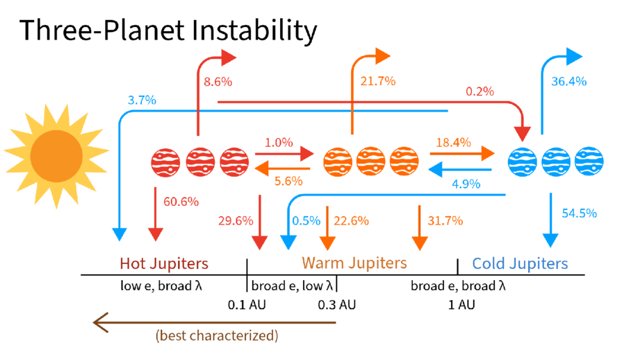
Each Jupiter-size planet in the galaxy falls into one of three distinct categories: hot, warm, or cold. A new study suggests that despite the apparent differences between these populations, they may have all formed from the same underlying dynamical process: a game of pool played at planetary scales.

A Diversity of Jupiters

Though our solar system has only one Jupiter-size planet, elsewhere in the galaxy we have found three different species of these massive gas giants. Cold Jupiters closely resemble their namesake and orbit far from their host stars; hot Jupiters are the opposite and are found whipping around their stars on extremely close-in orbits. In between these are the warm Jupiters, which tend to orbit in the intermediate space between 0.1 and 1.0 au.

A rendering of a star with lots of spots and flares with a planet in the foreground.

An artist’s depiction of a hot Jupiter. These planets orbit extremely close to their host stars, but likely got to their locations by scattering inward from more distant orbits. [NASA/JPL-Caltech]

Though these three populations are defined by their orbital distances, they differ from each other in other ways as well. For example, hot Jupiters almost never have nearby companions; if there are any other planets circling the same star, they’re usually far-out cold Jupiters. They can also orbit in pretty much any direction, including opposite the direction of their star’s spin, and are usually on perfectly circular orbits. In contrast, warm Jupiters often have friends nearby, are much more aligned with their stars’ spins, and can have modest eccentricities.

Given these differences, it’s often thought that each of these populations arrived at its current location through different dynamical processes and that the history of the warm Jupiters is likely quite different from the history of the hot Jupiters. However, a new study led by Julia Esposito (Georgia Institute of Technology) has proposed an alternative view. Maybe these populations, though they appear different now, were all created by the same process: planet–planet scattering.

Virtual Planetary Billiards

A cartoon of Jupiters at different distances from the sun with labelled arrows flowing inwards and outwards from each.

A schematic showing where different planets ended up as a function of where they scattered from during their evolution. Click to enlarge. [Esposito et al. 2026]

Esposito and collaborators set up 1,500 virtual planetary systems with three massive planets each, then simulated how the orbits evolved before probing the final configurations. In crucial contrast to previous simulation studies, the team initialized their Jupiters across a range of different distances and included the effects of tides sapping energy from orbits of planets that got too close to their host stars.

At the end of the simulation, the team surveyed the digital carnage. Almost every virtual system ended with only two planets after either ejecting one away from the star or having two planets collide. But, remarkably, the remaining two-planet systems looked tantalizingly similar to what we actually observe, with a mix of hot, warm, and cold Jupiters. Even more exciting, the end populations were highly correlated to where the violent scattering event took place.

For example, the warm Jupiters were almost all produced by “warm scattering” simulations, where the scattering took place between 0.1 and 1.0 au. The planets that survived the simulations and ended up as warm Jupiters matched all of the properties of the real warm Jupiter population: they had nearby companions, were moderately eccentric, and were mostly aligned with their stars. The hot Jupiters, meanwhile, were almost all produced by “cold scattering” events where the flybys happened far from the star and resulted in one planet hurtling inwards. These also matched all of the observed properties of real hot Jupiters.

The researchers concluded that planet–planet scattering can produce both the warm and hot Jupiter populations so long as you let the planets scatter from a variety of different distances. This exciting theoretical insight, if correct, would mean that astronomers could stop searching for different pathways to create each population. Happily, this model also provides testable predictions, and the authors lay out how the theory could be supported or disproven with additional data. Through virtual experiments like these, astronomers continue to build up an understanding of how the wide range of planetary architectures observed across the galaxy came to be.

Citation

“Unified Formation Channel of Hot and Warm Jupiters via Planet–Planet Scattering,” Julia Esposito et al 2026 ApJL 1003 L3. doi:10.3847/2041-8213/ae61b0

The post Playing Pool with Planets appeared first on AAS Nova.

Simulations of Turbulent Mixing Close One Gap but Open Another

6 May 2026 at 17:00

illustration of a white dwarf surrounded by rocky debris

Nature sometimes behaves in ways that are difficult to recreate in simulations. New research tackles the computational challenge of turbulent mixing and rules out a commonly assumed source of data–model disagreement.

Mixing Up Stellar Interiors

What do Earth’s oceans, red giant stars, and white dwarfs have in common? These are all sites of thermohaline mixing, a form of turbulent mixing that takes place when there is a vertical gradient in both temperature and chemical composition. For example, in Earth’s oceans, water near the surface is warmer and saltier than water in the depths below, setting up an unstable situation prone to mixing.

thermohaline mixing simulation results

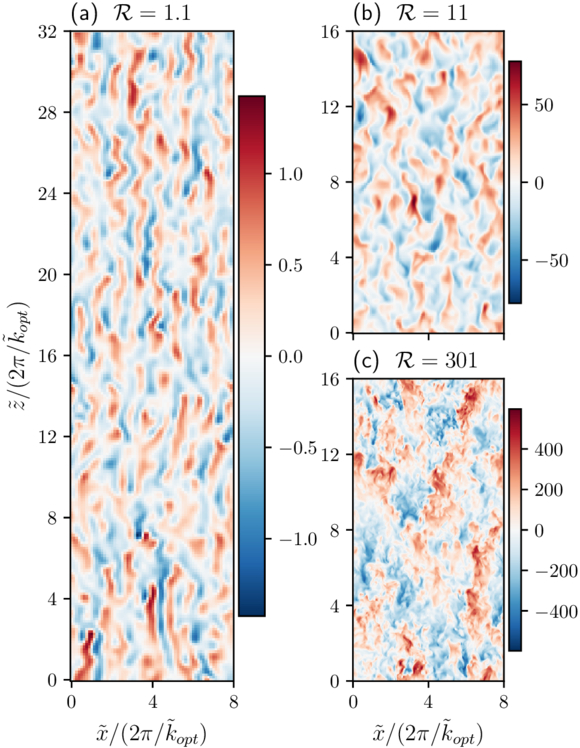
Examples of simulated thermohaline convection. These snapshots show the vertical velocity across a slice through the simulation volume. Click to enlarge. [Fraser 2026]

Thermohaline mixing has been explored in simulations to explain the evolution of red giants’ surface abundances, as well as how quickly rocky debris that accretes onto a white dwarf is absorbed into the star. However, effectively modeling this process in the interiors of stars has proven difficult.

One of the most important parameters for modeling mixing is the Prandtl number, Pr, which is the ratio of viscosity to thermal diffusivity (in other words, a way of describing whether momentum or heat diffuses more quickly within a fluid). For stellar interiors, Pr is around 10−6, but computational limitations have prevented modelers from setting this value lower than around 10−2. When tensions between models and reality arise, this gap between simulated and realistic Pr values is often assumed to be the source of the mismatch.

Bridging the Prandtl Number Gap

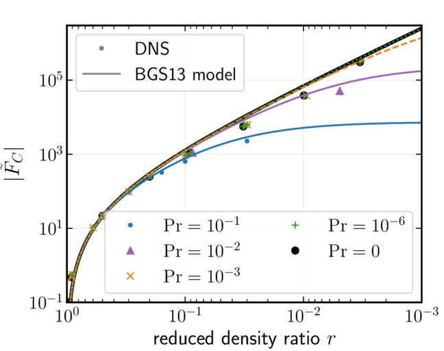
In a recent research article, Adrian Fraser (University of Colorado Boulder) aimed to test this assumption. Fraser carried out 3D simulations of thermohaline mixing, using a semi-implicit modeling technique that lowered the computational cost and allowed the simulations to probe Pr values of 10−1, 10−2, 10−3, 10−6, and 0.

comparison of simulations from this work and the benchmark model of thermohaline convection

Turbulent compositional flux as a function of reduced density ratio for the simulations from this work (DNS) and the benchmark model of thermohaline convection (BGS13). Click to enlarge. [Adapted from Fraser 2026]

By comparing these results against a benchmark model of thermohaline mixing, this exploration showed that adopting a realistic value of Pr doesn’t dramatically change the dynamics of the system — meaning that data–model incompatibilities can’t be swept under a Prandtl number–shaped rug and must instead be resolved by including additional physics.

Recreating Reality

Where does this leave modelers attempting to recreate the reality of stellar interiors? First, a silver lining of this investigation: Fraser found that setting Pr = 0 delivered nearly identical results to Pr = 10−6. This suggests that valid results can be attained in a much less computationally intensive way, since setting Pr = 0 lowers the complexity of the simulation. While simulations with Pr = 0 may not be appropriate for all scenarios, including systems with strong magnetic fields, it may provide a way forward in certain situations.

For modeling of red giants and white dwarfs, Fraser suggested that incorporating magnetic fields, stellar rotation, or additional sources of mixing may resolve the current discrepancies. In fact, some modeling work has shown that magnetic fields could entirely close the gap between observations and models for red giant surface abundances — suggesting that bringing models and observations into agreement may be within reach.

Citation

“Bridging the Prandtl Number Gap: 3D Simulations of Thermohaline Convection in Astrophysical Regimes,” Adrian E. Fraser 2026 ApJL 1001 L22. doi:10.3847/2041-8213/ae5796

The post Simulations of Turbulent Mixing Close One Gap but Open Another appeared first on AAS Nova.

In or Out? Using Balmer Emission to Distinguish Inflows from Outflows

1 May 2026 at 17:00

M33

Galaxies pull in and pump out gas as they form and evolve, but distinguishing between the two directions is tricky. A recent study used emission lines and dust absorption to try to pin it down.

Inflow or Outflow?

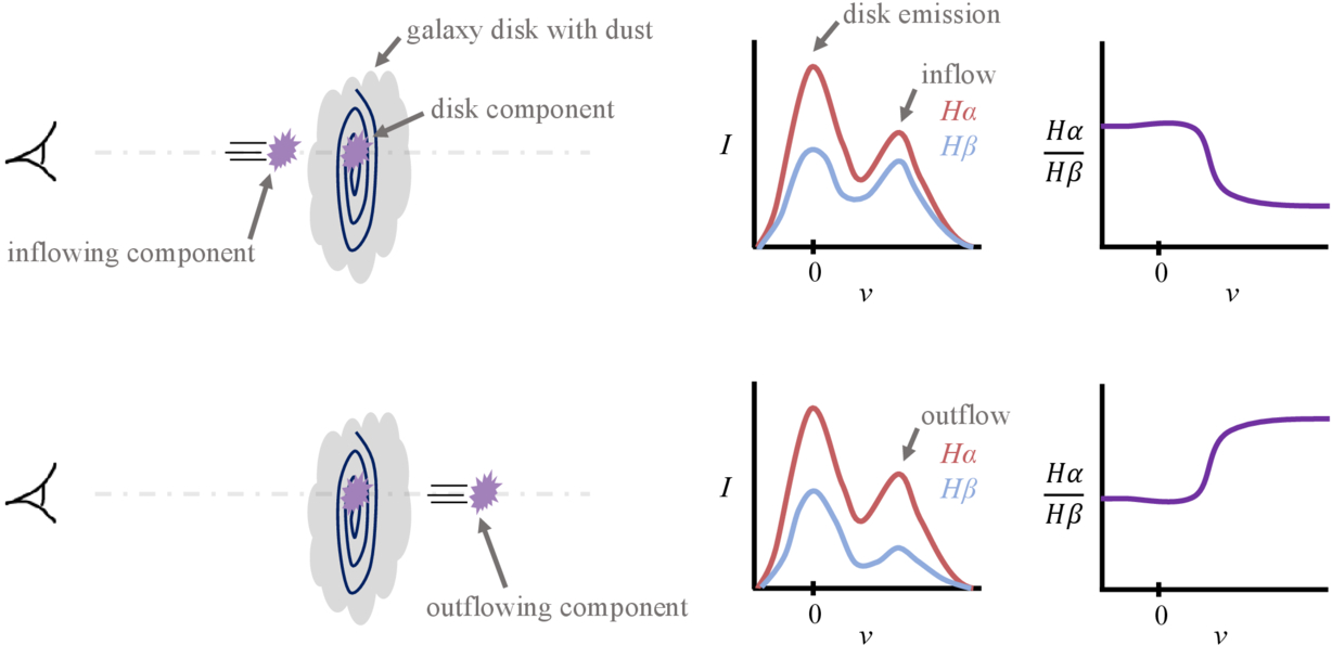
Throughout their lives, galaxies churn gas into stars, stars fuse new metals, supernovae blow enriched material back out, and the cycle repeats. To maintain this process and sustain star formation, a galaxy must fuel up by accreting gas from its surroundings. However, catching galactic gas accretion has proven difficult — both emission from gas falling into the galaxy (inflows) and gas blown out by supernovae (outflows) can appear blueshifted or redshifted along an observer’s sight line, depending on if the flowing material is in front of or behind the galaxy.

While direct evidence of inflows has been identified in the Milky Way, only a few direct detections of inflowing gas in other galaxies exist due to the degeneracy of inflow and outflow emission-line features. Relying on additional absorption measurements, some studies have teased out inflows in other galaxies, but these star formation fuel pumps remain overwhelmingly evasive. The angle at which we observe a galaxy also limits our ability to detect both inflows and outflows, with face-on galaxies best oriented to detect these shifted spectral features. How then do we uncover this critical component of a galaxy’s evolution?

Breaking Through with the Balmer Decrement

Balmer decrement diagram

A diagram illustrating the degeneracy in emission spectra of galaxies, with the top panel showing an inflowing component and the bottom panel showing an outflowing component. While the Hα emission is similar, the Hβ emission is more affected by extinction due to dust in the galaxy’s disk, making it possible to identify inflow versus outflow based on the Balmer decrement. Click to enlarge. [Sitaram et al 2026]

To try to break through the confusion between inflows and outflows, Meghna Sitaram (Columbia University) and collaborators explored how the strengths of hydrogen emission lines vary depending on the location of the emitting gas. Referred to as the Balmer decrement, the ratio between the Hα (redder) and Hꞵ (bluer) emission lines is sensitive to dust between the emitting gas and the observer. Because dust preferentially absorbs bluer photons, an inflow or outflow behind a galaxy is expected to have a higher Hα/Hꞵ ratio due to the intervening dust in the galaxy’s disk absorbing some of the Hꞵ emission.

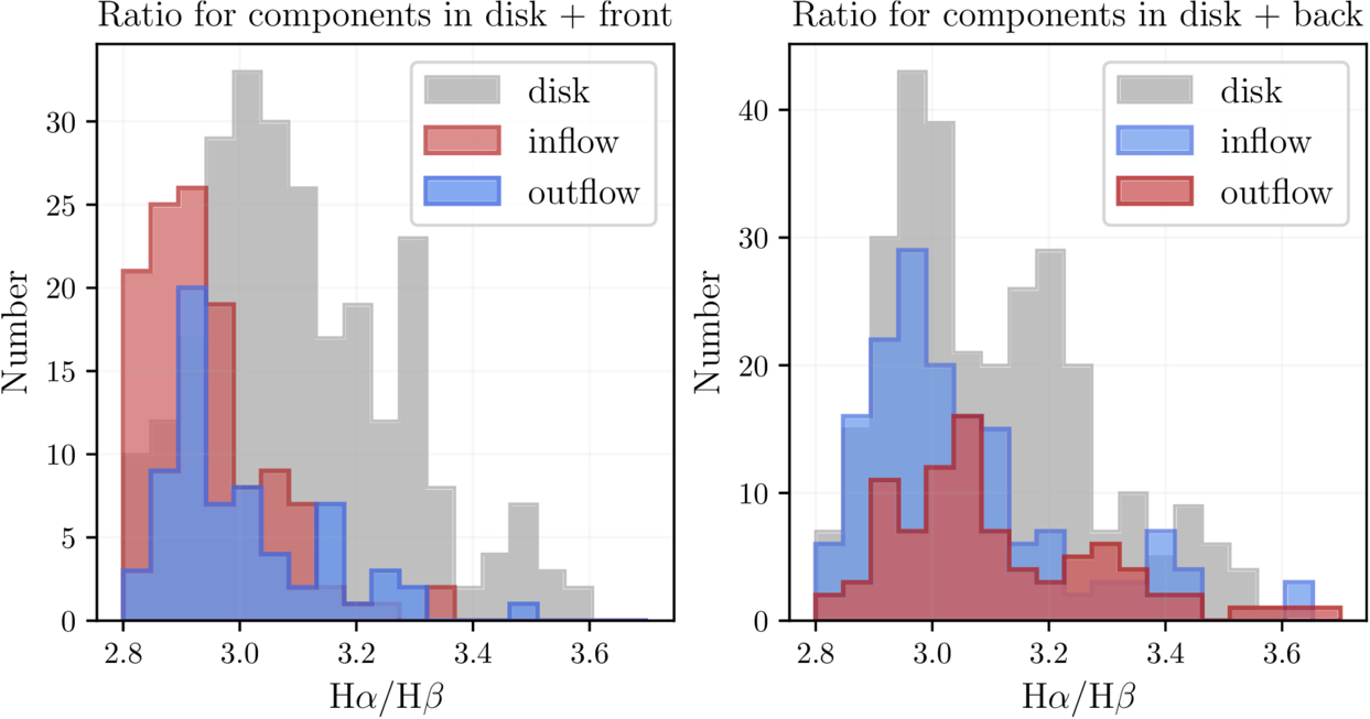
Testing this idea, the authors performed a hydrodynamic simulation of an isolated, face-on Milky Way–like galaxy and tracked inflows and outflows over a billion years. From the simulation, they extracted mock spectral observations to measure the ionized gas motions and Hα and Hꞵ emission lines along different sight lines throughout the galaxy. Separating gas components into three categories — inflow, outflow, and in the disk — the authors found that dust extinction does cause noticeable differences in the Balmer decrement depending on a component’s location with respect to the disk.

histograms

The distribution of Balmer ratios between different components in the interstellar medium and in front of the galaxy (left) and behind the galaxy (right). Material in front of the galaxy shows lower Hα/Hβ ratios. Click to enlarge. [Sitaram et al 2026]

Front Inflow Finds

What does this mean for identifying the inflows that provide galaxies with star-forming fuel? The authors reported that components in front of the galaxy — redshifted inflows and blueshifted outflows — tend to exhibit lower Hα/Hꞵ ratios compared to components behind the disk, aligning with the expectation that dust in the disk absorbs Hꞵ. In particular, these front inflows appear to be the most readily distinguished from gas in and behind the galaxy’s disk.

However, things get more complicated for gas behind the galaxy. Because the dust in the simulation is distributed nonuniformly in small clumps throughout the galaxy, it is difficult to distinguish between disk gas and gas behind the galaxy. While future simulations with improved dust modeling are necessary to resolve this issue, this study offers a useful method to distinguish inflow and outflow in dusty face-on galaxies.

Citation

“Identifying Signatures of Inflow onto Face-On Galaxies Using Balmer Decrement,” Meghna Sitaram et al 2026 ApJ 1001 87. doi:10.3847/1538-4357/ae5222

The post In or Out? Using Balmer Emission to Distinguish Inflows from Outflows appeared first on AAS Nova.

I Survived a Type Ia Supernova, and All I Got Was This Kick Velocity

17 March 2026 at 16:00

G272.2-3.2

Editor’s Note: Astrobites is a graduate-student-run organization that digests astrophysical literature for undergraduate students. As part of the partnership between the AAS and astrobites, we occasionally repost astrobites content here at AAS Nova. We hope you enjoy this post from astrobites; the original can be viewed at astrobites.org.

Title: Supernova Ia Remnants with M-Dwarf Surviving Companions
Authors: Kuo-Chuan Pan (潘國全), Pilar Ruiz-Lapuente, and Jonay I. González Hernández
First Author’s Institution: National Tsing Hua University
Status: Published in ApJ

Type Ia supernovae are important tools astronomers use to measure distances in space. Despite their important role as “standardizable candles,” their origins remain hotly debated. It’s long been theorized that a Type Ia supernova can develop from one of two pathways: the single-degenerate channel or the double-degenerate channel. In the single-degenerate channel, a white dwarf and a non-degenerate star (such as a red giant or main-sequence star like our Sun) orbit each other in a close binary system. The white dwarf accretes material from the outer surface of the non-degenerate star until it reaches a critical mass and explodes. The double-degenerate channel begins instead with two white dwarfs orbiting each other. Most explosion mechanisms from this channel result in the complete obliteration of the secondary, less-massive white dwarf. However, one theoretical explosion mechanism, called the dynamically driven double-degenerate double-detonation (D6) channel, might allow the secondary companion star to survive an explosion from a double-degenerate Type Ia supernova.

Generally, due to the immense energy from a supernova explosion, we expect these surviving companion stars to be “kicked” away from the blasts at high velocities. Fortunately, astronomers have found evidence of these surviving companion stars. As covered in a previous Astrobite, three hypervelocity white dwarfs have been found in Gaia data and traced back to the locations of double-degenerate Type Ia supernovae. Given the prevalence of Type Ia supernovae, however, astronomers are led to question why we haven’t seen many more of these candidates. It’s additionally important to wonder what similar “runaway” companions might look like for the single-degenerate channel.

Recent observations by the Gaia spacecraft near the supernova remnant G272.2-3.2 show an M-dwarf star, MV-G272, with an unusually high velocity around 240 km/s and a trajectory tracing back to the center of the supernova remnant. Is it possible for this M dwarf to be the runaway companion to the remnant’s original supernova? The authors of today’s article look at simulations of potential companion stars from single-degenerate Type Ia supernovae and compare their results to this observed potential companion candidate.

Because this work focuses on the potential for M-dwarf companions, the authors explored a range of simulated companion-star masses and radii characteristic of M dwarfs: 0.5, 0.6, and 0.7 solar mass and 0.396, 0.454, and 0.483 solar radius, respectively. To make these models, they used the stellar evolution code Modules for Experiments in Stellar Astrophysics (MESA) to construct and evolve a number of simulated stars with these specifications.

After setting up the models in MESA, they used the magnetohydrodynamics code FLASH to perform 2D and 3D simulations of the supernova explosion and the subsequent impact of the exploding star’s ejecta (or hot material) on its M-dwarf companion. After the explosion and impact were modeled, the companion star’s evolution was further followed in MESA.

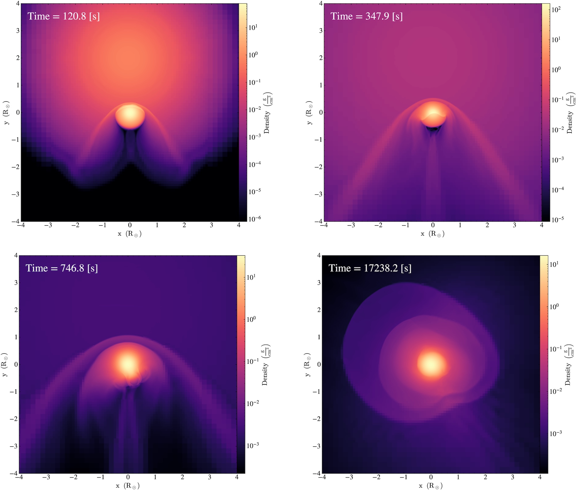
Figure 1 shows the density of the supernova’s ejecta, or exploding material, as it impacts the companion star. (You can think of this figure as if you were looking at the companion star out in space.) After roughly 100 seconds, you can see a bow shock develop around the top of the companion (or the “front” of the star) as it wraps around the companion. This impact causes significant compression of the companion star and rips away upwards of 50% the companion’s mass. The impact of this shock is what gives the companion star its “kick,” sending it hurtling through space.

simulations of supernova ejecta colliding with a star

Figure 1: Visual of the density of the companion star (center of each plot) and the supernova ejecta over time. In the top row of plots and the bottom-left plot, you can see the higher-density bow shock bent around the top (or front) of the companion star. In the bottom-right plot, you can see some of the supernova ejecta and unbound mass from the companion star settling around the companion star. [Pan et al. 2025]

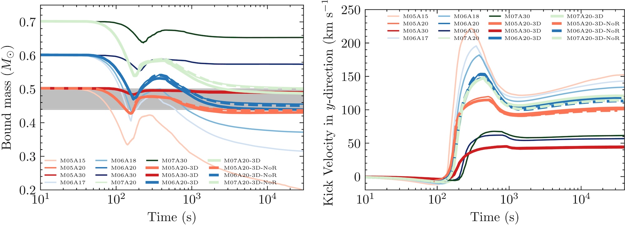
Because the authors explored a range of initial companion masses and distances between the primary and companion star, their results show some range. Figure 2 shows two important results: the evolution of the companion’s mass before and after the explosion (left plot), and the evolution of the companion’s kick velocity (right plot). The dip in mass around 100 seconds (102 s) indicates the impact of the bow shock. Even though the simulations model companions with a relatively narrow mass range (0.3–0.7 solar mass), there is considerable variation in the final masses after explosion. For example, the initial 0.5-solar-mass model ends up with anywhere between 0.07 solar mass (just 14% of its initial mass) and almost its full initial mass of 0.5 solar mass, depending on the distance between the companion and its exploding star.
plots of bound mass and kick velocity as a function of time

Figure 2: The different models shown in both plots indicate different initial masses and separation distances between the companion and the exploding star. Left: how the companion’s gravitationally bound mass evolves over time. The plot can be read left to right. The dip around 102 seconds indicates the impact of the supernova shock, which unbinds layers of the companion’s mass. Some of that mass becomes bound again to the companion after the shock passes. Right: how the companion star’s kick velocity changes based on initial mass and separation distance between companion and exploding star. The peak in values between 102 and 103 seconds indicates the impact, or “kick,” from the supernova. [Pan et al. 2025]

The results from this work generally show, predictably, that a companion closer to its primary star gets a bigger kick in velocity. These “kicks” range from about 50 km/s to 150 km/s. When added to the system’s initial velocity in space, it brings the total velocity of these companions into the 150–200 km/s range. This result is generally well aligned with the observed velocity of MV-G272, which was roughly 240 km/s.

Notably, runaway companion stars of these Type Ia supernovae seem to retain information from the initial explosion. Given the final velocities of these companions, astronomers might be able to figure out the companion’s initial mass and trace back its trajectory to the system it originated from. Overall, the fact that MV-G272 has a trajectory that tracks back to the center of a supernova remnant makes it a good companion candidate. These results support the feasibility of M-dwarf runaway companions from single-degenerate Type Ia supernova systems. Now that we know what these companions might look like — and how fast they can be going — astronomers can hopefully better search for these high-velocity stars in the future.

Original astrobite edited by Catherine Slaughter.

About the author, Mckenzie Ferrari:

I’m currently a PhD student in the geophysical sciences program at the University of Chicago. While I now study the atmosphere and oceans of Earth, most of my previous research focused on simulations of Type Ia supernovae and galaxy formation and evolution. In my free time, I foster cats for a local organization, enjoy cooking, and can often be found running along Lake Michigan.

The post I Survived a Type Ia Supernova, and All I Got Was This Kick Velocity appeared first on AAS Nova.

Ia’m Just Getting Started: A Type Ia Supernova’s First Day

24 February 2026 at 17:00

G299.2-2.9

Editor’s Note: Astrobites is a graduate-student-run organization that digests astrophysical literature for undergraduate students. As part of the partnership between the AAS and astrobites, we occasionally repost astrobites content here at AAS Nova. We hope you enjoy this post from astrobites; the original can be viewed at astrobites.org.

Title: The First Day of a Type Ia Supernova from a Double-Degenerate Binary
Authors: Gabriel Kumar, Logan J. Prust, and Lars Bildsten
First Author’s Institution: University of California, Santa Barbara
Status: Published in ApJ

Much like distance markers along the highway, Type Ia supernovae have long been used as distance indicators in space. These supernovae were originally theorized to form in binary systems. In this system, a white dwarf (a dense, collapsed remnant of a star) steals surface material from a non-degenerate star like our Sun and then explodes. Because of the initial conditions and properties of those two stars, the explosion would shine with the same intrinsic brightness regardless of the binary system’s location in space.

Research and observations, however, show that this is not entirely true; not all Type Ia supernovae are equally luminous. There are various theories regarding the different formation scenarios and explosion mechanisms that might create a Type Ia supernova. Developing ways to sleuth out the origins of these systems can be useful because it may tell us more about their luminosity.

One emerging theory of formation is the “double-detonation scenario.” In this case, two white dwarfs exist in a binary system. The more massive primary (the “accretor”) steals material from the less massive white dwarf secondary (the “donor”). After the primary steals the donor’s outer thin shell of helium, the helium surrounding the accretor detonates. This explosion induces a shock wave that travels into the dense core of the accretor and causes another detonation. The two detonations — one on the surface and one in the core — produce enough energy to explode the star into a supernova, a powerful stellar explosion. When the material from the exploding star reaches its companion star, it forms a mysterious, conical wake within the gaseous material, or “ejecta,” expelled from the accretor. This wake might be an important clue for distinguishing a supernova’s origins.

Since these explosions are incredibly powerful and would be difficult (and dangerous!) to perform in a lab, astronomers turn to computer simulations to model these events. Hydrodynamical simulations, in particular, are helpful for researchers because they model how fluids “flow” by solving complex equations that are too tricky to do by hand. (Remember that stars are just balls of gas, and hence fluid!) The authors of today’s article ran hydrodynamical simulations of the explosion and subsequent evolution of the ejecta from a double-detonation scenario.

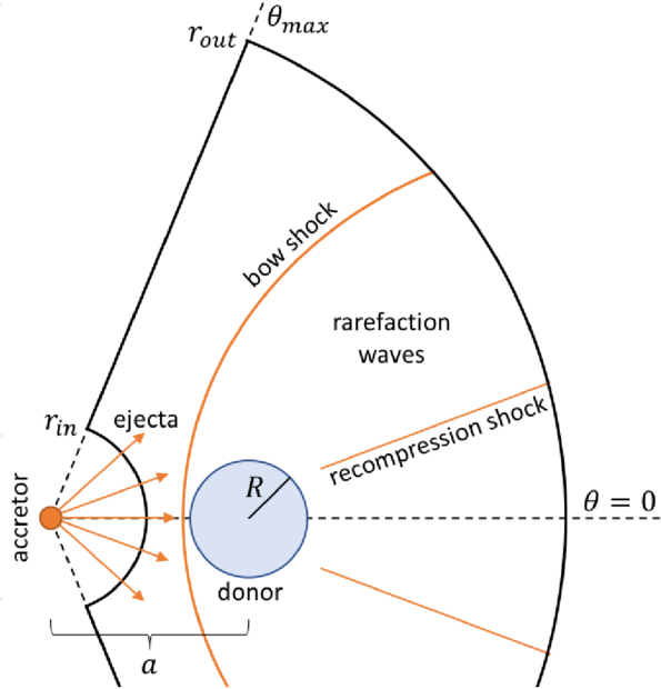
In the diagram of the team’s setup (see Fig. 1), you can see a “bow shock.” This shock is from the wave produced in the accretor’s detonation and is bowed since it bends around the donor star. This shock moves quickly through the cone of ejecta, modifies its structure, and leaves clues within the ejecta as it settles.

schematic of the simulation setup

Figure 1: A visual schematic of the simulation setup. The accretor is the exploding star, which produces a “bow shock” from the detonation. The bow shock and recompression shock modify the structure of the ejecta, which fills the space between rout and rin. The ejecta is full of gaseous stellar material. [Kumar et al. 2025]

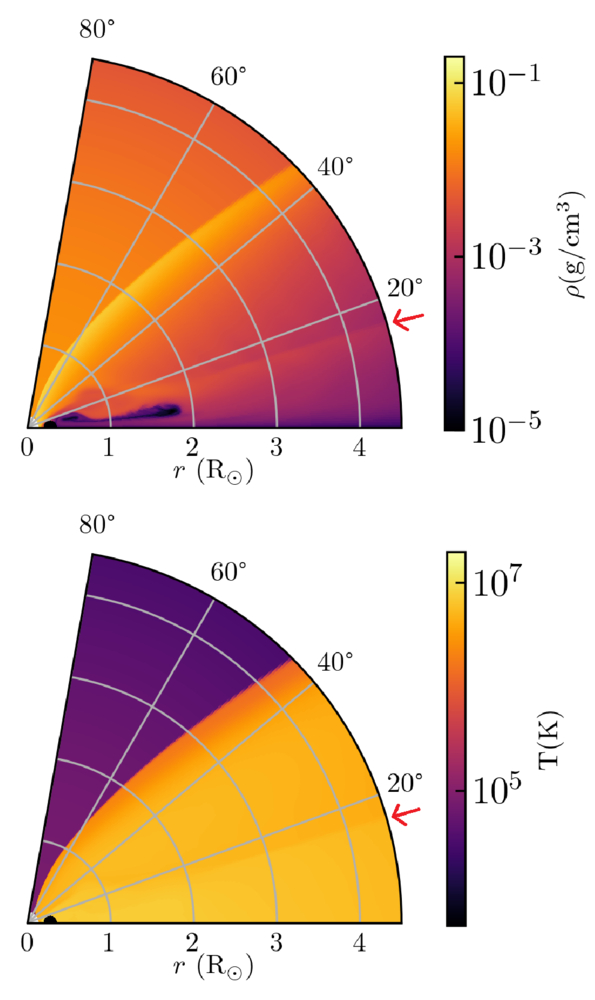
After simulating 1,000 seconds after the explosion, the authors recreated a high-density, low-temperature “wake” from the shock. You can see imprints of this wake in Fig. 2, as denoted by the red arrow.
visual slice of the simulated ejecta

Figure 2: A visual “slice” of the ejecta surrounding the donor star just 200 seconds after detonation. The bottom-left corner (r = 0) has a faint white spot, indicating the donor. The density (top) and temperature (bottom) of the ejecta are shown. The faint line marked by the red arrow indicates the secondary shock from the explosion, highlighting changes in both density and pressure. [Kumar et al. 2025]

Once they were able to produce this wake, the authors evolved the ejecta over time to see what the radiation from this material might reveal. They discovered that the “shocked,” or compressed and heated, ejecta flew out much further than the unshocked ejecta (see Fig. 3).
simulation snapshot at 2 hours of simulation time

Figure 3: A slice of the simulation taken later, at 2 hours of simulation time. The ejecta in the shocked region has flown out farther than the ejecta in the unshocked region. Note that the horizontal scale has changed from Figure 2. [Kumar et al. 2025]

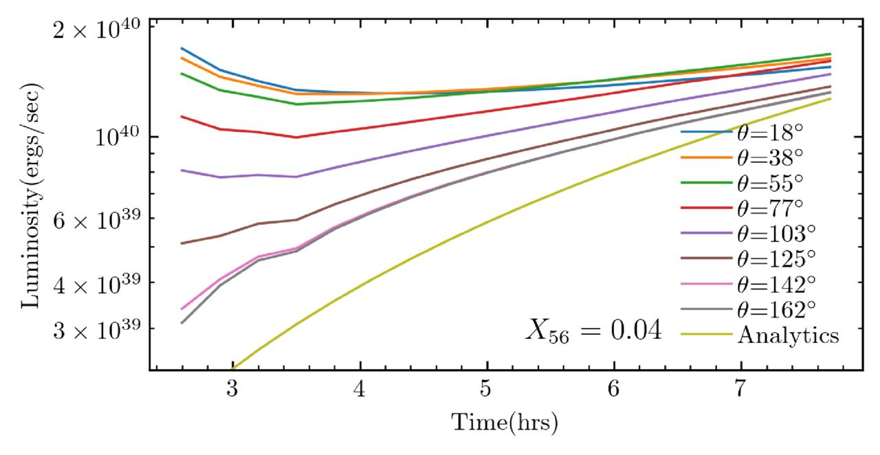
This ejecta can be seen from different viewing angles, influencing an observer’s measurement of the explosion’s luminosity. The strongest features of the wake are visible up to about 55 degrees, while some effects can still be seen up to about 140 degrees — almost half of the sky (see Fig. 4). Overall, an observer’s position relative to the explosion axis might change their reported luminosity of the explosion. The authors estimate that this wake might cause Type Ia supernovae from a “double-detonation” scenario to appear up to 15% fainter, depending on the observer’s viewing angle. Therefore, if scientists use Type Ia supernovae as cosmic distance indicators, their calibrations might be slightly off. This isn’t the best news for those using measurements of Type Ia supernovae to measure the expansion rate of the universe.
plot of luminosity versus time after detonation of a supernova

Figure 4: A comparison of luminosity vs. time over the course of 6 hours shortly after detonation. The different lines indicate different viewing angles from the axis of explosion. The line “Analytics” describes a light-curve prediction by Piro (2012) for a supernova that was not shock-heated. The luminosities for this model span almost one order of magnitude. [Kumar et al. 2025]

We’ve talked a lot about the accretor and ejecta in this scenario, but what might happen to the donor star? One idea is that the donor star is “kicked” away by the high velocity of the blast. In this simulation, the authors were able to calculate a “kick” velocity, or speed imparted by the blast to the donor star, that was much higher than estimates from other detonation models. One observed Type Ia supernova, SN 2021aefx, is believed to have the fastest observed ejecta to date. The mechanism that today’s authors modeled might explain how the ejecta of this event got its super-fast “kick.”

While there is always more work to be done, this work presents a first step at identifying double-detonation Type Ia supernovae from early observations. With an influx of observations from new observatories, like the Vera C. Rubin Observatory, we should expect to see many more early supernova detections.

Original astrobite edited by Ansh Gupta.

About the author, Mckenzie Ferrari:

I’m currently a PhD student in the geophysical sciences program at the University of Chicago. While I now study the atmosphere and oceans of Earth, most of my previous research focused on simulations of Type Ia supernovae and galaxy formation and evolution. In my free time, I foster cats for a local organization, enjoy cooking, and can often be found running along Lake Michigan.

The post Ia’m Just Getting Started: A Type Ia Supernova’s First Day appeared first on AAS Nova.

We Have Visitors: Interstellar Material from Nearby Debris Disks

6 February 2026 at 17:00

'Oumuamua

Traversing the galaxy from places yet known, a few interstellar objects have taken a quick dip into our solar system. These objects have inspired a frenzy of questions regarding their origins and paths that led them here. A recent study took to nearby planet-forming stellar systems as possible launching posts.

Interstellar Object Origins

As 3I/ATLAS was first spotted entering the solar system in July 2025, all eyes turned to the curious interstellar visitor. Just the third interstellar object astronomers have observed, 3I/ATLAS joins 1I/ʻOumuamua (2017) and 2I/Borisov (2019) in capturing our attention and igniting many questions regarding their origins and journeys to our corner of the Milky Way. While astronomers have characterized these objects’ compositions, sizes, and paths through the solar system, the mechanisms by which these objects leave their origin systems and travel the galaxy before arriving here are not well constrained. 

These three large bodies are just part of the interstellar material visiting the solar system — spacecraft have detected an influx of small interstellar dust particles, and while not yet directly confirmed, interstellar meteoroids burning up in Earth’s atmosphere are possible. This loose material likely originates in dusty, planet-forming disks (debris disks) around stars — rubble kicked out into interstellar space, sending chemicals, organic compounds, and perhaps even the precursors of life to other nearby systems. Understanding the origins and trajectories of such material will allow us to investigate planet formation and how developing systems may impact their environments.

Deliveries from Debris Disks

Debris disks offer ideal testbeds for tracing small bodies and dusty material through the galaxy. Interactions with large planets in debris disks can launch loose material like planetesimals and dust into interstellar space. To explore how debris disks may drive interstellar visitors to our solar system, Cole R. Gregg and Paul A. Wiegert (The University of Western Ontario) simulated how much material the 20 nearest debris disks would contribute to the interstellar object population of our solar system.

sky projection for particle arrival directions

Arrival direction on the sky for particles that reach the solar system from the 20 debris disks studied here. The arrival locations for 1I/ʻOumuamua, 2I/Borisov, and 3I/ATLAS are shown for comparison. Click to enlarge. [Gregg and Wiegert 2025]

The authors modeled the trajectories of ejected material from each debris disk within a simulated Milky Way, running the simulations backward and forward in time to trace the ejecta over 100 million years. These simulations show that material from each of the 20 systems is currently expected to be within our solar system. For interstellar objects (≥100 meters), the simulations predict that about two objects from these debris disks are currently within the inner solar system.

Trickier to spot, smaller meteoroids (≥200 microns) that would appear as meteors in Earth’s atmosphere are also expected. The only way to observationally confirm interstellar origins for meteors is based on how fast they are moving relative to the material in our solar system, or their excess velocities. Based on the simulations, many of these smaller particles have low excess velocities, making them observationally difficult to distinguish from bound solar system objects.

Observational Connections and Expectations

'oumuamua zoom in plot

Zoomed-in view focusing on the direction where 1I/ʻOumuamua entered the solar system. The interstellar object falls near the arrival directions of particles from HD 38858 and HD 166. Click to enlarge. [Gregg and Wiegert 2025]

How do these simulations compare to observations? From their analysis, the authors identified where the interstellar material from each debris disk would first enter the solar system. Comparing these to the entry locations of 1I/ʻOumuamua, 2I/Borisov, and 3I/ATLAS, ʻOumuamua appears near the entry locations for debris from HD 166 and HD 38858. (2I/Borisov and 3I/ATLAS had no such match up in this sample of debris disks.) However, tracing ʻOumuamua’s travel backward, its closest approaches to these systems are about 32 and 18 light-years away, respectively — likely too far to have originated from either system but still a clear proof of concept that we can place interstellar objects near potential systems of origin. 

Where are the expected interstellar meteoroids? Current meteor detectors including the Canadian Meteor Orbit Radar (CMOR) and the Global Meteor Network (GMN) search the sky for incoming material. While the simulations predict hundreds of meteoroid-sized particles from each debris disk currently in the inner solar system, the small collecting area of CMOR and the limiting size of grains detectable by GMN statistically require decades of observations to detect even a single interstellar meteoroid. Thus, the lack of detections thus far is not surprising, but with advanced instrumentation, discoveries of more interstellar particles and objects are imminent.

Citation

“A Catalogue of Interstellar Material Delivery from Nearby Debris Disks,” Cole R. Gregg and Paul A. Wiegert 2025 PSJ 6 309. doi:10.3847/PSJ/ae284f

The post We Have Visitors: Interstellar Material from Nearby Debris Disks appeared first on AAS Nova.

Standing on a Sub-Neptune

5 November 2025 at 17:00

A rendering of a blue planet in the foreground and a small bright star in the background.

Astronomers often assume that sub-Neptune exoplanets have magma oceans hiding beneath their atmospheres. New research suggests that this might not always be the case.

Puzzling Type of Planet

In the 30 years since the discovery of the first exoplanet, astronomers have come to appreciate that many of the most common planets in our galaxy look nothing like the worlds in our solar system. One type of planet in particular appears to be ubiquitous despite not appearing in our own cosmic neighborhood: sub-Neptunes. As their name suggests these planets are slightly smaller than Neptune, but still much larger than Earth or what we’d expect from a planet composed mostly of rock.

Four planets side by side ordered by increasing size. From left to right, they are Earth, TOI-421 b, GJ 1214 b, and Neptune.

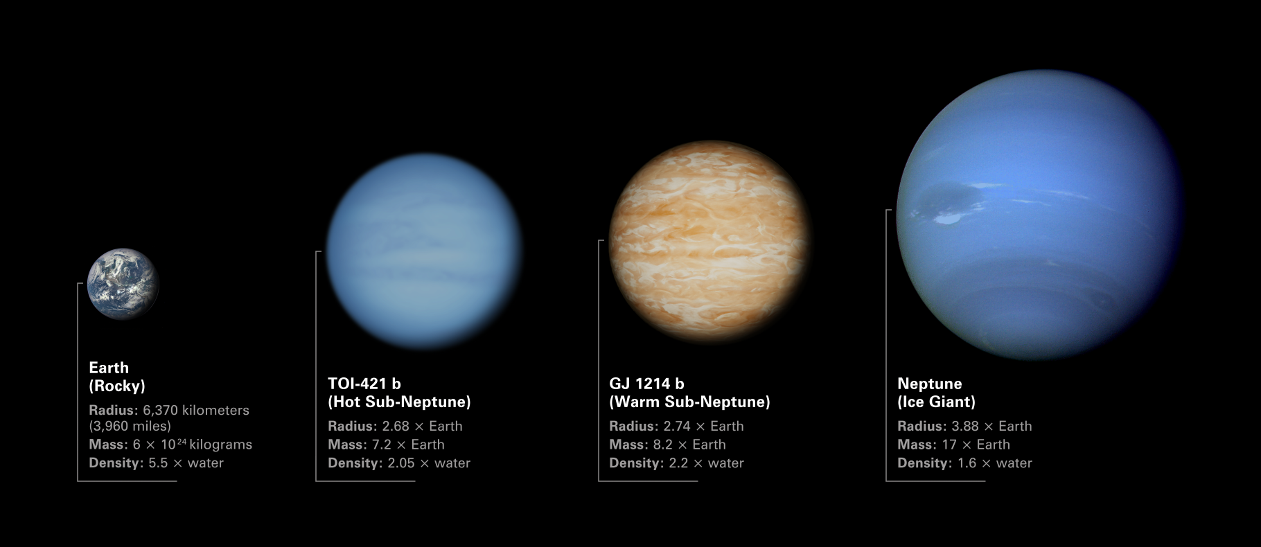
An illustration of how two sub-Neptunes mentioned in this study (TOI-421b and GJ 1214b) compare with planets in our solar system. Click to enlarge. [NASA, ESA, CSA, Dani Player (STScI)]

What sub-Neptunes are made of and how they formed are still mysteries under active investigation by the research community. It is possible that these worlds are mostly rocky and sport puffy, light atmospheres over their surfaces; it’s also possible that these worlds are watery, and that most of their mass comes from heavy, steamy atmospheres. In most cases, though, it’s assumed that the high pressures and temperatures at the surfaces of these worlds foster a permanent, fiery magma ocean.

This key assumption that there’s no solid surface to stand on influences our models about how these planets cool and evolve over time. However, new research led by Bodie Breza (University of Maryland) suggests that this premise might not always be appropriate.

Solid Ground

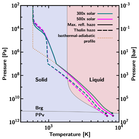
To test the assumption that every sub-Neptune has a magma ocean, Breza and collaborators simulated hundreds of thousands of feasible exoplanet interiors and atmospheres. Each simulation slightly tweaked various characteristics, like the surface temperature or the planet’s total mass, then checked whether the temperature and pressure conditions at the planet’s surface would leave any rocks in solid or liquid form.

phase diagram for a common rocky material

A phase diagram for a common rocky material MgSiO3. The various lines show different model pressure–temperature profiles for the sub-Neptune GJ 1214b, while the circles indicate the location of the atmosphere/surface boundary. All circles fall into the “solid” part of the phase diagram, indicating that GJ 1214b likely has a solid surface. [Breza et al. 2025]

Somewhat surprisingly, the team found that about a third of the models they simulated had solid, not magma, surfaces. They found there were two distinct ways to solidify the magma and create a firm shell. First and most intuitively, if the surface temperature falls low enough, the magma will simply freeze. Second and more intriguingly, they found that a planet can also suppress a magma ocean if its atmosphere is heavy enough to drive up the surface pressure beyond the solid–liquid threshold.

This latter result is particularly insightful in light of recent JWST observations that suggest many sub-Neptunes have heavy atmospheres. These new models suggest that these worlds might have solid surfaces, and that models attempting to explain their compositions should be tweaked to account for this finding. In these early days where astronomers are still puzzling out the most basic properties of these strange worlds, research like this demonstrates the power of using advanced theoretical modeling to help interpret our cutting-edge observations.

Citation

“Not All Sub-Neptune Exoplanets Have Magma Oceans,” Bodie Breza et al 2025 ApJL 993 L46. doi:10.3847/2041-8213/ae0c07

The post Standing on a Sub-Neptune appeared first on AAS Nova.

Planetary Hide and Seek

1 October 2025 at 17:00

illustration of a planetary system

Editor’s Note: Astrobites is a graduate-student-run organization that digests astrophysical literature for undergraduate students. As part of the partnership between the AAS and astrobites, we occasionally repost astrobites content here at AAS Nova. We hope you enjoy this post from astrobites; the original can be viewed at astrobites.org.

Title: The Gap–Giant Association: Are Planets Hiding in the Gaps?
Authors: Caleb Lammers and Joshua Winn
Authors’ Institutions: Princeton University
Status: Published in ApJ

The Kepler space telescope played an almost decade-long game of hide-and-seek. After nine and a half years of operation, Kepler detected more than 2,700 planets outside of our solar system primarily by using the transit method, which is particularly efficient at detecting planets that orbit close to their host stars. Astronomers have also been detecting planets with the radial velocity technique, which is better at finding larger planets at longer orbital periods. By looking for planets with both the transit and radial velocity techniques, astronomers can look for both close-in and far-out planets to paint a more complete picture of other solar systems in our galaxy.

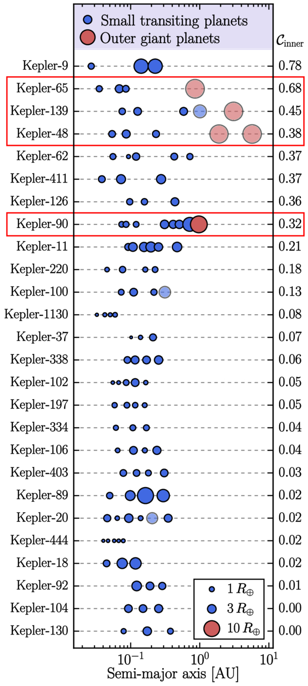
Using the Kepler Giant Planet Survey, the authors of today’s article found that among the 26 systems with three or more transiting planets, four were found to also have an outer giant planet. They quickly noticed that instead of an evenly spaced out inner system of planets, every single one of these four systems with the outer giant planets revealed a notable gap between two of their inner planets. They dubbed this phenomenon the “gap–giant association” — in other words, when an outer giant planet exists in a planetary system, there is evidence of a large gap between two of the inner planets, as shown in Figure 1. This pattern has been observed before, but there has been little theoretical work to explain the effects of outer giants on orbital spacings. In today’s article, the authors ask the question: are there planets inside the gap hiding from us? To address this, they conduct simulations to see if (a) these systems can host a hiding planet in their gaps without becoming dynamically unstable and (b) if such a planet can remain hidden when looked for with the transit method.

Plot of the orbital spacing of planets

Figure 1: Orbital spacings of systems in the Kepler Giant Planet Survey with three or more transiting planets in the inner planetary system. The parameter C is a metric denoting the regularity of orbital spacings, where a smaller value would indicate a more uniform spacing. The four systems of interest all have large orbital gaps between two adjacent inner planets, and therefore high values of C. [Lammers & Winn 2025]

Close Your Eyes and Count to N

The authors of today’s article model these four systems (Kepler-48, Kepler-65, Kepler-90, and Kepler-139) with a planet added to their gaps and use an N-body simulation (i.e., fancy physics calculations that track how planets gravitationally interact) to evolve the systems over time and evaluate their long-term stability. They find that each of these injected planets has a high survival rate, which means that each of these four systems could stably host an additional ~2–20 Earth-mass planet in its gap for billions of years without falling apart. The authors then calculated whether the outer giants could “hide” these theoretical gap planets by tilting the planets’ orbits enough so that they would not be detectable with the transit method. In order to do this, the outer giant would have to exert a large enough gravitational force on the gap planet to cause it to precess at a rate independent of its neighbors, allowing its orbital inclination to grow. However, they found that the outer giant planets are either too far away or not massive enough to do the job.

Only one system, Kepler-90, has an outer giant that could potentially tilt the gap planet’s orbit enough for it to fly under the radar if the giant were also on a modestly inclined orbit. However, previous detections of Kepler-90’s outer giant suggest that its orbit is well-aligned with those of the inner system, making this hypothesis implausible. They therefore concluded that it is unlikely that planets between ~2 and 20 Earth masses are hiding within these gaps.

Seeking Out Another Option

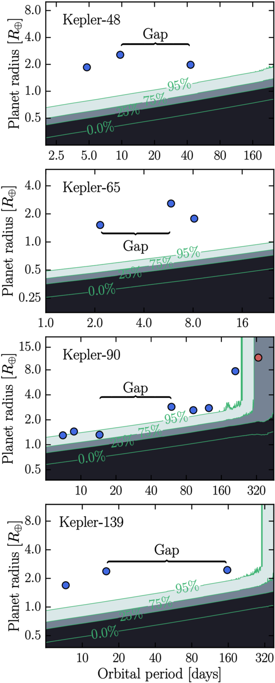
Before completely abandoning this hypothesis, the authors propose that maybe the gaps do contain planets, but they’re just too small for Kepler to detect. They calculate the detection efficiencies as a function of planet radius and orbital period for each of the four systems and find that planets smaller than about ~0.5–1 Earth radius could have gone unnoticed (as shown in Figure 2). While this would make these systems slightly unusual (most multiplanetary systems have relatively uniform planet sizes), it’s not completely impossible. However, they don’t rule out the possibility that these gaps are truly empty, and that the presence of an outer giant could prevent planets from forming in certain regions or disrupt their orbits after formation. While it is hard to draw any firm conclusions with a sample size of four systems, this study highlights how much we still don’t understand about planetary system architecture, and therefore planetary formation and evolution.

Plots of transit detection efficiency as a function of planetary radius and orbital period

Figure 2: Transit detection efficiency as a function of planetary radius and orbital period for each planetary system. The inner planets and location of the gap are overplotted. The darker contours show regions where Kepler is not sensitive to detecting planets. In order to avoid detection, the planets in each of these systems would have to be much smaller relative to their neighbors, except for the Kepler-90 system, where a hidden planet would only have to be marginally smaller. This suggests that there could exist a demographic of exoplanets that are evading detection within these gaps. [Lammers & Winn 2025]

Though the Kepler mission has come to an end, ongoing radial velocity surveys will continue to expand the sample of systems like these four so astronomers can get a clearer picture of what’s behind this gap–giant association.

Original astrobite edited by Annelia Anderson.

About the author, Tori Bonidie:

I am a 5th-year PhD candidate studying exoplanet atmospheres at the University of Pittsburgh. Prior to this, I earned my BA in astrophysics at Franklin and Marshall College where I worked on pulsar detection as a member of NANOGrav. In my free time you can find me cooking, napping with my cat, or reading STEMinist romcoms!

The post Planetary Hide and Seek appeared first on AAS Nova.

Scars from a Black Hole

10 September 2025 at 17:00

A spiral of bright material circling a black core.

Simulations suggest that there should be a million stars in our galaxy that once wandered so close to a supermassive black hole that they were nearly destroyed. What are the long-term effects of this encounter, and could astronomers observe the scars of these near-death experiences?

Moths to a Flame

center of the Milky Way

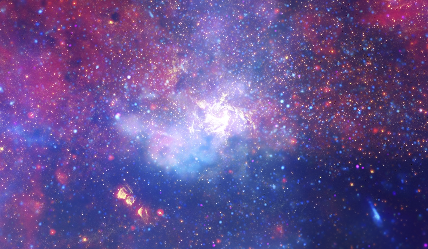
This infrared and X-ray image of the Milky Way’s center shows a swirl of hot gas surrounding Sagittarius A*, our galaxy’s central supermassive black hole. [NASA, ESA, SSC, CXC, STScI]

The center of our galaxy is a dangerous place to be a star. Like mosquitoes drawn to a light, millions of stars swarm around the supermassive black hole named Sagittarius A*, packing themselves in tight and kicking one another onto wild, eccentric, and ever-changing orbits. Every 100,000 years or so, one of these stars gets an unlucky push and finally gives in to the black hole’s irresistible pull. A nudge from a neighbor will send it hurtling beyond the point of safety, and in one intense flyby, it’ll be ripped apart by Sagittarius A*’s immense gravitational field.

Simulations suggest that most of the time, these hapless stars are not completely destroyed by their close encounters with the black hole. In principle, then, there should be about a million “survivor” stars wandering near the center of our galaxy. But, what would these survivors look like? And with careful measurements, could we tell them apart from their regular, unscathed counterparts?

Simulating a Star’s Worst Day

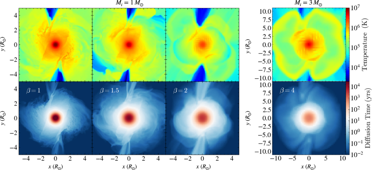
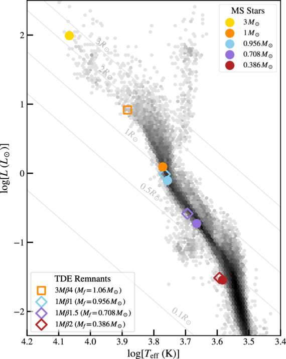
Recently, a team of astronomers led by Rewa Clark Bush (University of California Santa Cruz, Cabrillo College, Wesleyan University) tackled this question. First, the team needed to simulate a terrible day for a hypothetical star: the day it passes closest to the black hole. To compute what happens to the star in those intense couple of hours, they used an open-source hydrodynamic code called FLASH to track the state of the star in granular detail.

An 8-panel figure showing complex, asymmetric patterns of gas around a dense core.

Temperatures (top row) and diffusion timescales (bottom row) of four stars soon after their closest approach to the black hole. Click to enlarge. [Bush et al. 2025]

Then, once the star (or what was left of it) managed to flee back to safety, the team froze the simulations and took stock. They found that depending on the initial size of the star and the distance of its closest approach, the black hole stripped away anywhere from a few percent to almost two thirds of the star’s mass. The researchers then fed the stars into another code called MESA to simulate how the disturbed stars would settle into a new equilibrium and evolve over billions of years.

Back on Track

Plot comparing disturbed and undisturbed stars

Comparison of the original undisturbed stars (filled circles), the stars after a black hole encounter (open symbols), and other stars with different initial masses (black points). Click to enlarge. [Bush et al. 2025].

The team found that although these unlucky stars likely glow tens to hundreds of times brighter than usual after their flyby, this period of enhanced brightness lasts less than 100,000 years. For our galaxy, this translates to 1–10 stars currently in the galactic center that have been brightened by an encounter with a supermassive black hole.

Eventually, though, these stars pretty much return to a new normal. Though these stars would have had slightly different colors and luminosities had they not encountered the black hole, they end up looking similar to undisturbed stars with the same final mass.

Although detailed spectroscopic measurements of these remnants might reveal a strange composition thanks to all the stirring that happened during the flyby, it’d be hard to tell anything happened to these stars otherwise. Ultimately, life goes on, even for stars that were nearly destroyed by the most massive creature in the galaxy.

Citation

“Black Hole Survival Guide: Searching for Stars in the Galactic Center that Endure Partial Tidal Disruption,” Rewa Clark Bush et al 2025 ApJL 990 L7. doi:10.3847/2041-8213/adefde

The post Scars from a Black Hole appeared first on AAS Nova.

Escaping the Dust Trap: Simulations of Dust Dynamics in Protoplanetary Disks

25 July 2025 at 17:00

Through detailed simulations of gas and dust, a recent study revealed that the behavior of dust within protoplanetary disks is a bit more complex than previously assumed.

Dust Traps in Protoplanetary Disks

As a planet forms within a protoplanetary disk — dust and gas orbiting a new star — tidal interactions between the budding body and the dusty material surrounding it can create pressure bumps where dust builds up. These dust traps appear as rings in observations of protoplanetary disks.

Dust traps are thought to play a critical role in the disk’s evolution and the early stages of planet formation. Dust traps may prevent solid material from migrating inward, starving the inner disk and impeding planet growth interior to the trap. These reservoirs may also serve as a chemical barrier, keeping volatile materials like water from moving to the inner regions of a disk.

While a perfect dust trap completely isolates material from the rest of the disk, recent observations and 2D simulations have shown that dust traps may be a bit more permeable — leaking smaller sized grains, mixing material, and changing the disk’s appearance. However, these results only account for two dimensions of the complex three-dimensional environment in which dust traps reside. Thus, 3D hydrodynamical simulations are necessary to provide more realistic details of dust dynamics within planet-hosting protoplanetary disks. 

Dusty Simulations

Dust-gas density ratios for 3d models at 1500 orbits

Z-axis averaged dust–gas density ratios (top) and dust–gas surface density ratios for the 3D simulations after 1,500 orbits. For the simulations with higher diffusion and lower planet mass, there is clear leaking of dust beyond the dust trap ring (edges marked with dotted red lines). Click to enlarge. [Huang et al 2025]

In a recent study, Pinghui Huang (Chinese Academy of Sciences; University of Victoria) and collaborators performed multiple 2D and 3D numerical simulations of gas and dust within a protoplanetary disk with a forming planet. The simulations varied the mass of the planet and the level of turbulent diffusion — how well material and energy flow and mix within the gas. These variations allowed the authors to explore how dust traps behave within different types of systems. 

The simulations showed that the embedded planet will perturb the gas and dust, producing density shocks that create gaps and, subsequently, pressure bumps where dust traps coalesce. From their analysis, the authors found that dust traps become leakier at higher levels of diffusion and when the embedded planet is lower in mass. Essentially, if the gas flows and mixes more efficiently, the perturbations of the planet are erased more quickly, and if the planet is sufficiently small, its ability to disrupt the disk is much weaker. Dust remains coupled to the gas, flowing through these weak traps without becoming stuck. Additionally, the 3D simulations show higher amounts of leakage compared to the 2D simulations, which the authors attributed to the asymmetric and complex vertical geometry of the disk.

Trapping over time.

Flux-trapping ratio (left) and mass-trapping ratio (right) as a function of time for the 2D (top) and 3D (bottom) simulations. The higher-mass planet in Model A causes more flux and mass-trapping than the lower-mass planets and more turbulent systems. Additionally, the 3D simulations show significantly lower flux and mass-trapping than the 2D simulations. Click to enlarge. [Huang et al 2025]

Implications and Comparison to Observations

What then are the consequences of leaky dust traps? In planet formation theory, dust traps determine the mass at which a planet creates a sufficient pressure bump that isolates small pebbles and dust exterior to its orbit. For perfect dust traps, this isolation of material from the planet and inner disk creates a clear chemical distinction between the inner and outer disk. However, as shown by the 3D simulations, dust traps are imperfect, allowing small particles to filter through; the authors suggest this may mean that the growing planet slows but does not stop the migration of solid materials in a disk.

Recent observations of protoplanetary disks reveal the presence of larger volatiles within the inner disk. Specifically, the disk PDS 70 shows water emission in its inner disk despite having two confirmed giant planets orbiting in the outer disk. Without leaky dust traps, volatiles like water would be trapped in the pressure bumps created by these planets. However, as the authors have shown, the complex reality of dust dynamics within protoplanetary disks allows heavier elements to leak through, enriching the inner disk. Further observations and detailed 3D simulations will allow astronomers to understand the extent of leaky dust traps and reveal the realistic conditions driving early planet formation.

Citation

“Leaky Dust Traps in Planet-Embedded Protoplanetary Disks,” Pinghui Huang et al 2025 ApJ 988 94. doi:10.3847/1538-4357/addd1f

The post Escaping the Dust Trap: Simulations of Dust Dynamics in Protoplanetary Disks appeared first on AAS Nova.

Featured Image: Following Photons Through Curved Spacetimes

16 June 2025 at 17:00

Today’s featured image is a beautiful representation of how simulated images of active black holes are made. In a recent research article, a team led by Aniket Sharma (Indian Institute of Science Education and Research Mohali) introduced Mahakala, a new ray-tracing algorithm that expertly tracks photons as they navigate the warped spacetimes surrounding black holes. Mahakala is named for the Egyptian deity who, as Sharma and collaborators describe, is “believed to be the depiction of absolute black, and the one who has the power to dissolve time and space into himself.” The image above shows a simulated accreting black hole at a wavelength of 1.3 millimeters, which is the same wavelength used by the Event Horizon Telescope to view the supermassive black holes at the center of the Milky Way and the galaxy Messier 87. The dotted lines streaming off to the right represent the paths that photons took on their way to the viewer as they curved around the black hole, which is visible among the forest of lines. In this representation, the color of each dot shows the synchrotron emission generated at that point in three-dimensional space. The team hopes that Mahakala, which can be run quickly and easily from a Python Jupyter notebook, helps make the complex world of general relativistic magnetohydrodynamics simulations more accessible. You can try it for yourself or learn more from the article linked below.

Citation

“Mahakala: A Python-Based Modular Ray-Tracing and Radiative Transfer Algorithm for Curved Spacetimes,” Aniket Sharma et al 2025 ApJ 985 40. doi:10.3847/1538-4357/adc104

The post Featured Image: Following Photons Through Curved Spacetimes appeared first on AAS Nova.

❌