❌

Reading view

AAS 248: Day 4

Andromeda Galaxy

Editor’s Note: This week we’re at the 248th AAS meeting in Pasadena, CA. Along with a team of authors from Astrobites, we will be writing updates on selected events at the meeting and posting each day. Follow along here or at astrobites.com for daily summaries, or follow @astrobites.bsky.social on Bluesky for more coverage. The usual posting schedule for AAS Nova will resume on 22 June

Table of Contents:


Plenary Lecture: Ian Roederer, The Ultraviolet Path to the Origin of the Elements (by Susanna Kohler)

When the universe first formed, the only elements present were the three lightest — hydrogen, helium, and lithium. Today, there are 118 confirmed chemical elements that make up the periodic table. So where did the heavier elements come from, when were they first created, and what can they tell us about the first stars that formed in the universe? In the final plenary of AAS 248, Ian Roederer (North Carolina State University) walked us through how ultraviolet observations are the key to understanding the origin of the elements.

We know that hydrogen, helium, and lithium were cycled through the earliest stars in the universe, where fusion and other processes produced the first heavy elements that were spit back out into the cosmos when these stars ended their lives as supernovae. According to Roederer, within just the first two or three generations of stars, every element with stable or long-lived isotopes had already been created. For the heaviest of these elements, the dominant source is likely a process called r-process nucleosynthesis, in which a rapid burst of neutrons bombards atomic nuclei, resulting in the quick capture of the neutrons to form very massive nuclei that subsequently decay to stable isotopes.

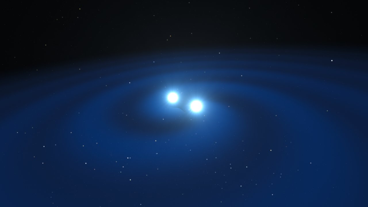
illustration of a neutron star merger

Illustration of two neutron stars approaching a merger, emitting gravitational waves as they draw closer together. [ESO/L. Calçada/M. Kornmesser; CC BY 4.0]

The conditions needed for r-process nucleosynthesis are too extreme to reproduce in a laboratory on Earth, so we rely on models and observations of the cosmos to better understand it. We know that to get a rapid burst of neutrons, you need some sort of explosive event — and, in fact, the first example of an r-process event caught in the act was GW170817, the first detected neutron star–neutron star merger.

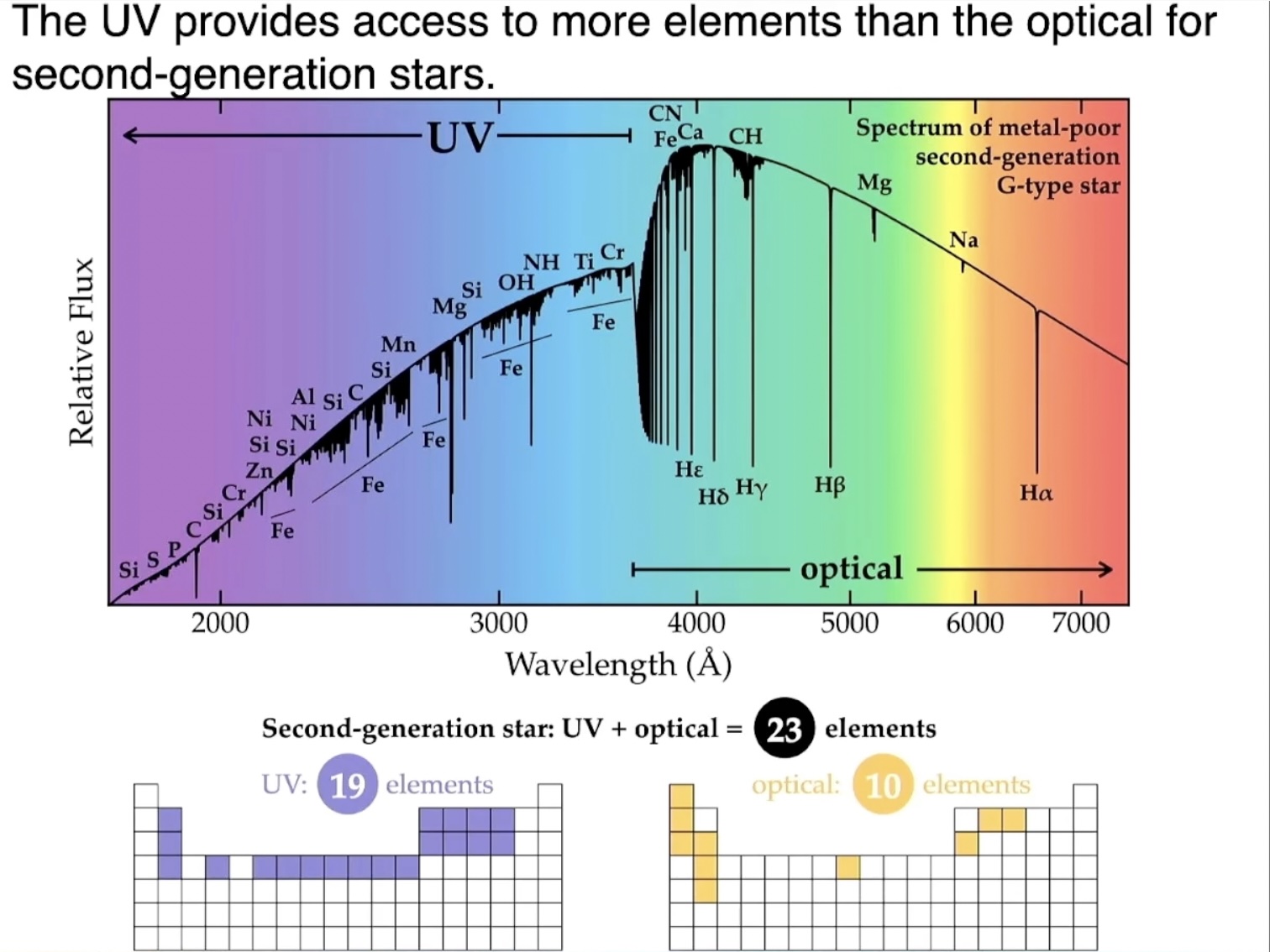
But remember all those news headlines about how binary neutron star mergers produce gold and platinum? Roederer points out that these were all inferred results — we didn’t actually observe direct evidence of gold and platinum in the aftermath of this explosion. That’s because it’s very difficult to detect the spectroscopic emission lines of heavy elements. To do so effectively, Roederer argues, requires high-resolution ultraviolet (UV) spectroscopy. He showed that in a cool star, high-resolution UV spectra provide a 50% increase in the number of elements you can detect. The heaviest of elements are only detectable with spectra in the UV range.

A stellar spectrum shows a large number of metal lines identified in the UV, as compared to fewer lines in other wavelengths. Text at the top of the slide reads "the UV provides access to more elements than the optical for second-generation stars."

An example spectrum for a second-generation star shows how the UV is critical for identifying a broad range of elements. [Roederer 2026]

Roederer walked us through some of the insights we can gain into the production of the heaviest nuclei found in nature when we use a combination of UV and optical spectroscopy. He also gave examples of what we can learn about even some of the lighter elements like phosphorus or boron when we have high-resolution UV spectroscopy to reveal the presence of these elements in low-metallicity stars.

Roederer ended his talk with a look ahead at the future of UV spectroscopy and the path to the universe’s first stars. Right now, the only mission we have that produces high-resolution UV spectroscopy is Hubble. NASA’s next big flagship mission with a high-resolution spectrograph, the Habitable Worlds Observatory (HWO), will be transformational in the ability to detect — or verify the absence of — heavy elements in stellar atmospheres. An observatory like HWO will provide our best shot at identifying low-mass, metal-free stars that survive from the first generation of stars in our universe. As Roederer concluded, “The future of studying the origin of the elements is bright in the UV.”

You can read Astrobites’s interview with Ian Roederer here.

The post AAS 248: Day 4 appeared first on AAS Nova.

  •  

AAS 248: Day 3

double supernova remnant

Editor’s Note: This week we’re at the 248th AAS meeting in Pasadena, CA. Along with a team of authors from Astrobites, we will be writing updates on selected events at the meeting and posting each day. Follow along here or at astrobites.com for daily summaries, or follow @astrobites.bsky.social on Bluesky for more coverage. The usual posting schedule for AAS Nova will resume on 22 June.

Table of Contents:


Plenary Lecture: Eliza Kempton, Common Worlds, Uncommon Complexity: Sub-Neptune and Super-Earth Atmospheres in the JWST Era (by Lexi Gault)

Eliza Kempton began her talk addressing the undergraduates in the room, showing the meeting website from AAS 200, which she attended as an undergraduate in 2002. Searching this page, there were no presentations on exoplanets — a stark difference from the boom of exoplanet science that we see 24 years later at AAS 248, marking how significantly a field can transform from the start of your career.

Situating us outside of the solar system, Kempton showed the quintessential mass–period plot of all 6,000+ detected exoplanets thus far. Strikingly, we have discovered new types of planets that are not seen in our own solar system, but uncovering exoplanet populations is heavily skewed due to detection limits. While it is much easier to find large planets closely orbiting their stars, occurrence rate studies have shown that small planets on close-in orbits are much more common and typically come in two sizes: gas-rich sub-Neptunes and rocky super-Earths. However, actually deciphering their compositions relies on detailed studies of their atmospheres, which is the primary research work Kempton dove into.

How do we study exoplanet atmospheres? Thankfully, JWST provides the wavelength range and collecting area necessary for observing the minute details in exoplanet atmospheres. Beginning with sub-Neptunes, Kempton laid out four important takeaways from recent work coming from her team:

  1. Sub-Neptune atmospheres composed of heavier elements and molecules are common.
  2. Clouds and hazes are pervasive for planets that get a moderate amount of light from their host star. Early JWST observations showed signatures that may point to soot formation in sub-Neptune inner atmospheres; this soot can rise, making the upper atmosphere we observe hazy.
  3. Sub-Neptune atmospheres may provide a window into their interiors. Observed atmosphere compositions may indicate no solid planetary surface, but rather magma, water, and/or gas that can mix more readily with the upper atmosphere.
  4. Tying atmospheric observations to formation scenarios is still a challenge. Constraints on planets’ bulk composition has not provided clear answers.

Moving down to super-Earths, Kempton introduced the idea of the cosmic shoreline — the empirical relationship between planetary escape velocity and stellar irradiation shows a stark dividing line between planets with and without atmospheres in our solar system. Does this concept of a cosmic shoreline exist for exoplanets? Kempton highlighted three takeaways for the study of super-Earth atmospheres:

  1. Spectroscopy of super-Earth atmospheres presents degeneracies in determining their characteristics. A featureless spectrum could be due to the presence of heavy molecules and clouds, or it could just mean the planet has no atmosphere.
  2. Thermal emission is a powerful tool for identifying candidate atmospheres. The eclipse depth of a transiting planet is directly related to the day-side temperature of the planet. Planets with and without atmospheres will have different day-side temperatures — hotter without an atmosphere, cooler with an atmosphere.
  3. Many (but not all) transiting super-Earths are bare rocks. 

Clearly, JWST has allowed astronomers to make significant progress in understanding exoplanet composition and subsequently their possible formation and evolutionary histories. Kempton ended with reminding us where we came from 24 years ago — the field of exoplanet science has boomed, and we can wonder how much we’ll continue to uncover in the next 24 years.

Return to Table of Contents.


Press Conference: Stars Reshaping Galaxies: Clusters, Feedback, and Explosive Aftermaths (Briefing video) (by Niloofar Sharei)

This press conference brought together four very different views of star-forming environments: the most distant galaxy cluster caught strongly lensing a background galaxy, the dense young star clusters tucked inside the rings of nearby galaxies, the extreme feedback physics inside the closest luminous infrared galaxy merger, and the first known pair of supernova remnants born from a binary star system.

A New Era of Galaxy Cluster Analysis at Cosmic Noon: JWST’s View of a Distant Galaxy Cluster

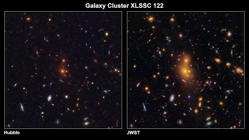
Kyle Finner (IPAC/Caltech), presented the discovery of strong gravitational lensing in XLSSC 122, the most distant known galaxy cluster, seen as it was about 10.3 billion years ago. When the team got their JWST imaging back, they noticed bright blue arcs around the brightest cluster galaxy, a clear signature of strong lensing from a background galaxy sitting in just the right place behind the cluster. Using those arcs, the team measured the radial dark matter profile and found that XLSSC 122 is much more centrally concentrated than cosmological simulations predict. To check whether the cluster itself is unusual, they combined the JWST result with multiwavelength data. All of those tracers show an elongated structure pointing the same way as the dark matter, which is a strong sign that XLSSC 122 is a merging cluster. But mergers usually lower concentration rather than boost it, so the question of why this early cluster looks so concentrated is still open. The team plans to follow up with more strong-lensing measurements. | Press release

This two-panel image shows a distant galaxy cluster

This two-panel image shows a distant galaxy cluster as it has been observed by NASA’s Hubble Space Telescope and JWST. [NASA, ESA, CSA; Kyle Finner (Caltech/IPAC) Image processing: Robert Hurt (Caltech/IPAC-SELab)]

Hidden Gems in the Hearts of Nearby Galaxies: Evolution of Young Massive Star Clusters in Circumnuclear Rings

Sajia Shahrin Neha (University of Kentucky) presented a study of young massive clusters in the circumnuclear rings of two nearby galaxies: NGC 3351, a normal spiral, and NGC 1097, which hosts an active galactic nucleus. Young massive clusters are extreme star-forming systems that pack hundreds of thousands to millions of stars into a small region, and the ring-shaped star-forming zones around these galactic nuclei provide exactly the kind of dense gas and dust reservoir these clusters need. Because the clusters are heavily obscured, optical, ultraviolet, and infrared light cannot pass through cleanly, so Neha and collaborators turned to radio continuum imaging with the Atacama Large Millimeter/submillimeter Array and the Very Large Array, which can see through the dust. Their team identified 53 young massive cluster sources across the two rings. They also placed them on an evolutionary sequence: heavily embedded “starless” clumps, newborn clusters that are just starting to become visible, and older “exposed” clusters that have already burned through much of their gas. All evolutionary stages are present in both galaxies, regardless of whether the host has an active nucleus. | NRAO press release | U. Kentucky press release

Dusty and Over-Pressured: Measuring Stellar Feedback in the Closest Luminous Infrared Galaxy

Deb/Debosmita Pathak (The Ohio State University/IPAC) presented new measurements of pre-supernova stellar feedback in NGC 3256, the closest luminous infrared galaxy and a merger between two roughly Milky Way–mass galaxies. NGC 3256 forms stars about 60 times faster than the Milky Way, which makes it a useful nearby laboratory for the intense, clumpy star formation that dominated the early universe. Using JWST plus multiwavelength data, the team measured feedback pressures around roughly 1,700 young star clusters and compared them with what we see in quieter, normal star-forming galaxies. The results break the standard picture in two ways. First, the feedback and interstellar medium pressures in NGC 3256 are about a hundred times higher than what is typical in normal star-forming galaxies. Second, the dominant feedback mode is different: instead of warm ionized gas pressure doing most of the work, ultraviolet and infrared radiation pressure on dust dominates in these much dustier environments. Even at these much higher pressures, most clusters are still over pressured relative to their surroundings, meaning radiation is strong enough to drive expansion against a dense ambient interstellar medium. | NRAO press release | OSU press release

Unveiling the First Binary-System Supernovae

Miltiadis Michailidis (Kavli Institute for Particle Astrophysics and Cosmology (KIPAC)/Stanford University/SLAC National Accelerator Laboratory) closed the session with the discovery of what appears to be the first known supernova remnant pair born from a binary star system. The starting point is IC 443, one of the best-studied supernova remnants and one of the brightest gamma-ray sources in the sky, thanks to its interaction with a dense nearby molecular cloud. Recent eROSITA observations showed that the faint X-ray “shell” long noticed next to IC 443 is in fact a second, overlapping supernova remnant. The question was whether the two are physically related or just a chance alignment on the sky. They used 15 years of Fermi gamma-ray data and modeled and subtracted IC 443’s contribution and uncovered a distinct, hidden gamma-ray source associated with the new remnant.

The gamma-ray emission is strongly spatially segregated: its northern boundary, where it overlaps the same molecular cloud that IC 443 illuminates, is dominated by accelerated protons colliding with dense gas, while its southern boundary is dominated by accelerated electrons. The team also showed that the optical filament along the northern boundary is a radiative shock that has cooled past the point of efficient particle acceleration. Combined with the fact that both remnants sit at the same distance (about 6,000 light-years), and that a population-synthesis run with a million massive binaries reproduces the observed separation and age difference, the team argues that the two remnants are the remains of a true binary pair. | Press release

Return to Table of Contents.


Plenary Lecture: George Helou, The Cosmic Infrared Window: Photons, Technology, and People (by Kerry Hensley)

George Helou (Caltech) gave a sweeping overview of infrared astronomy over the past 40 years, including the impressive role of the Infrared Analysis and Processing Center, or IPAC, which is celebrating its 40th anniversary.

The infrared portion of the electromagnetic spectrum is broad, encompassing wavelengths from 1 to 1,000 microns. In that wavelength range, there’s a lot going on in our universe: redshifted emission from distant galaxies, stars revealed by the drop in dust extinction, rotational and fine structure lines, molecular transitions, and fully half of the radiation density in the universe.

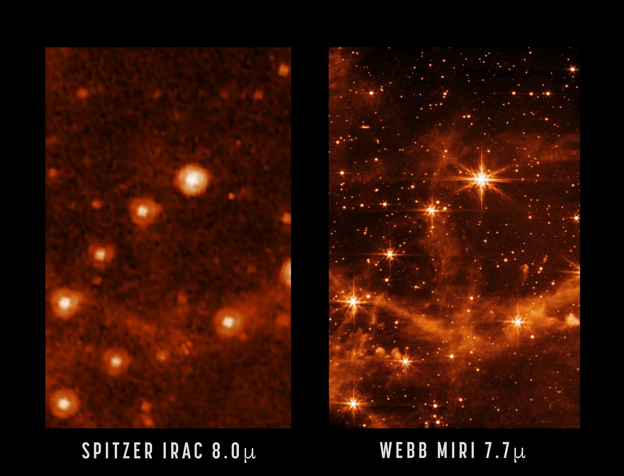
comparison of Spitzer and JWST images

An example of how infrared capabilities have improved over time. [NASA/JPL-Caltech; MIRI: NASA/ESA/CSA/STScI]

There have been many successful ground- and space-based infrared missions and surveys over the past four decades, starting with the Infrared Astronomical Satellite (IRAS), which proved the potential of infrared astronomy from space and set a new standard for making data accessible and well documented. Next, the Infrared Space Observatory (ISO) revealed the full span of infrared emission from objects like galaxies and gave researchers their first glimpse of H2 lines. The Two Micron All Sky Survey (2MASS) produced the first fully digital survey of the sky at high angular resolution, creating a dataset that is still widely used. The Spitzer Space Telescope, the Wide-field Infrared Survey Explorer (WISE), the Herschel Space Observatory, and the Planck satellite followed, bringing a slew of new and unexpected discoveries, and pushing the field of infrared astronomy to longer wavelengths.

Helou introduced a few science areas in which infrared missions have contributed greatly. First was the study of polycyclic aromatic hydrocarbons (PAHs), which are a class of molecules containing interconnected rings of carbon atoms. Thanks to infrared instruments, astronomers showed that various unassigned spectral features arose due to PAHs and that these molecules were important for the heating and cooling of the interstellar medium. As infrared instruments became more capable, observations showed how the fraction of carbon that is locked up in PAHs changes with metallicity and revealed novel species like deuterated hydrocarbon nanoparticles.

In the field of exoplanets, IRAS found evidence of excess infrared emission around Vega, hinting at a disk of debris that was later confirmed. (IPAC was instrumental in this discovery; the star Vega was being used for calibration, and the calibration wouldn’t converge because of the unexpected infrared excess.) Later, ISO used spectroscopy to investigate stellar debris disks and showed that they were similar in properties to solar system comets. Though Spitzer wasn’t initially expected to be used for exoplanet studies, the telescope made the first detection of photons from the surface of a planet and helped to discover several planets in the TRAPPIST-1 system. (Here, IPAC played an integral role again; instrument teams and flight engineers worked to ready the spacecraft for exoplanet observations by modifying the heaters on the spacecraft for pointing stability and finding “sweet spots” for photometric stability.) Today, JWST continues to advance the field with sensitive measurements of exoplanet atmospheres.

Finally, Helou touched on the work that IPAC has done to archive data. IPAC maintains the NASA/IPAC Extragalactic Database, or NED, which receives at least three queries per second. It’s also responsible for the Infrared Science Archive, data from which is used in more than 50% of research articles. IPAC also manages the NASA Exoplanet Archive, showing that the center isn’t limited to infrared astronomy!

As for the future of IPAC and infrared astronomy, it’s clear that there is much left to explore and lots of exciting work to be done; the Roman Space Telescope is scheduled to launch in a few months, and within a few years the Near-Earth Object Surveyor will follow. The Ultraviolet Explorer, for which IPAC will provide the UVEX Science Data Center, is slated to launch in 2030, and the PRobe far-Infrared Mission for Astrophysics (PRIMA) is under final review.

Read Astrobites’s interview with George Helou.

Return to Table of Contents.


Plenary Lecture: Carolyn Kuranz, Creating Astrophysical Conditions at High Energy Density Facilities (by Lucas Brown)

While astronomy and astrophysics are often considered primarily observational sciences, with most targets of interest being millions to trillions of miles away from us — Carolyn Kuranz’s plenary talk helped to challenge this idea, demonstrating how we can sometimes bring the heavens down to Earth with high energy density (HED) facilities. The basic idea behind Kuranz’s work, and the field of HED laboratory astrophysics more broadly, is that some extreme astrophysical environments, particularly plasmas, can indeed be studied in the lab by producing smaller-scale analogs — so long as we choose the right types of experiments.

Kuranz structured her talk around three big questions she commonly gets asked about her field: firstly, why would astronomers want to do laboratory experiments? Then, what defines the “high energy density” in HED astrophysics? And finally, how do we actually do these experiments in practice? Starting with the why, Kuranz notes that studying systems in astrophysics is inherently difficult as a result of the fact that they are far away, and theoretical models can suffer from a lack of data or missing physics. Experiments can bridge the gap here, providing the ability to collect more data on specific systems of interest, complementing both theoretical models and observations.

While this philosophy can apply to a variety of laboratory astrophysics areas, such as laboratory-based studies of the chemistry of planetary atmospheres, Kuranz focused specifically on the emerging role of HED laboratory astrophysics. Typically, high energy density refers to systems with more than 1 million atmospheres of pressure and temperatures above 1 million K. Generally, this means we’re in plasma territory. In some ways, it’s only natural that studies of these sorts of environments would eventually help astrophysicists, given that around 99.9% of the matter in the universe is in plasma form. Despite this, the laboratory astrophysics side of HED physics has really only emerged over the past 30 years, with its origins being traced to work out of Lawrence Livermore National Lab, the current site of the National Ignition Facility (NIF).

Today, the NIF is only one of a few dozen facilities in which HED laboratory astrophysics experiments are conducted. This is because the type of equipment needed to reproduce environments analogous to various astrophysical systems can vary greatly. This gets to Kuranz’s third question of how these experiments are conducted. The process begins by answering a set of questions, including: do the astrophysical and proposed laboratory environments obey the same governing equations (conservation of mass, momentum, etc.)? Is one able to re-scale the physical parameters in each system (timescale, size, density, pressure, etc.) in a way that retains relevant dynamics like viscosity, Reynolds number, and so on? Once these details have been nailed down, a researcher can assess what types of facilities they may need. For example, the NIF, which uses symmetrical arrangements of lasers to compress and heat up millimeter-scale pellets containing gases that can undergo nuclear fusion, provides a fairly natural environment for studying processes in the cores of stars, which are also hot, dense, and neutron-rich environments where fusion is actively occurring.

As for the future, things look promising for HED laboratory astrophysics — since the NIF achieved “ignition” in 2022, producing a net gain of energy from one of these pellet-crushings for the first time, a huge amount of interest and investment has been flowing into facilities studying HED physics. These facilities range from private companies working to achieve sustained nuclear fusion power generation to longstanding federal research centers working on understanding nuclear weapons and stockpile management, but they all provide astronomers with the opportunity to do what was once unthinkable: bring the universe’s most extreme environments down to Earth.

Return to Table of Contents.


Plenary Lecture: Cara Battersby, Our Galaxy’s Dynamic Center (by Niloofar Sharei)

Cara Battersby (University of Connecticut) used her plenary to walk us through her group’s ongoing effort to understand one of the most extreme environments in our own galaxy: the central molecular zone (CMZ), which is a dense, turbulent gas reservoir at the heart of the Milky Way. Her talk pulled together large surveys, new high-resolution zoom simulations, and machine-learning methods designed to bridge between the two.

She opened with the PRobe far-Infrared Mission for Astrophysics (PRIMA), the far-infrared probe mission concept she is a co-investigator on. This mission concept was developed in response to NASA’s recent billion-dollar probe mission call, and selection is expected later this year. PRIMA covers roughly 1.8–25 microns with imaging and spectroscopy, and galactic ecosystems make up about a quarter of its science case.

Battersby paused mid-talk to speak directly to early-career people in the audience about work-life balance, including bringing her daughter and sister with her to the meeting, and the SPARK program at UConn that supports women and underrepresented groups in physics. Her message: astronomy should be done from a place of joy, and visible work-life balance is something the community should be more open about.

Battersby framed the Milky Way as the natural laboratory for star formation across a huge range of environments, and briefly reviewed the ALMAGAL survey, which observed roughly 1,000 high-mass star-forming regions across the disk. But her main focus was the CMZ, which she argued is essentially a different kind of galaxy embedded inside our own. About 80% of all the dense molecular gas in the Milky Way sits in the CMZ, and its gas properties — density, turbulence, temperature, and pressure — are extreme compared to the rest of the disk. Because nearby starburst and high-redshift environments share many of these properties, the CMZ is the closest place we can actually resolve individual star-forming cores under conditions that resemble the early universe.

She showed that gas in the CMZ is extremely filamentary across all scales, and that the relationship between dense gas and star formation rate is unusual: when individual clouds in the CMZ actually form stars, they form them much like clouds elsewhere in the galaxy, but a large fraction of the dense gas in the CMZ never engages in star formation at all. Battersby argued that this is likely because so much of that gas is being shaped by flows toward the black hole and the strong turbulence and dynamics of the central environment, and it never cools and collapses into stars.

She closed with the simulation and machine-learning side of the program. Her group runs zoom simulations that can follow individual star-forming regions and can resolve down to CMZ scales while still capturing the full ~5 kpc bar driving gas inward. To extract more from these simulations than just side-by-side image comparisons, the team built a GPU-accelerated radiative transfer code that runs roughly 10,000 times faster than existing codes. They generate hundreds of thousands of synthetic observations and use them to train an encoder–decoder convolutional neural network that learns to predict the top-down structure of a region from the side-on view we actually observe. Applied to the CMZ, the network produces 3D reconstructions that are physically plausible and broadly consistent across independent training runs.

Read Astrobites’s interview with Cara Battersby.

Return to Table of Contents.

The post AAS 248: Day 3 appeared first on AAS Nova.

  •  

AAS 248: Day 2

NGC 2210

Editor’s Note: This week we’re at the 248th AAS meeting in Pasadena, CA. Along with a team of authors from Astrobites, we will be writing updates on selected events at the meeting and posting each day. Follow along here or at astrobites.com for daily summaries, or follow @astrobites.bsky.social on Bluesky for more coverage. The usual posting schedule for AAS Nova will resume on 22 June.

Table of Contents:


Helen B. Warner Prize Lecture: Kyle Kremer, Globular Clusters: Astronomical Factories of Gravitational-Wave and Electromagnetic Transients (by Lucas Brown)

Kyler Kremer (University of California, San Diego) kicked off day two of AAS 248 with a “dynamic” talk on the complex interactions and environments that exist within globular clusters — the most massive category of stellar clusters, which can contain upwards of one billion stars. Because of the extreme stellar density of these environments, they are thought to be good factories of systems ranging from accreting white dwarfs to millisecond pulsars, which are often spun up to high speeds via accretion from companion stars. Such accretion, whether onto pulsars or other compact objects, can often generate bright X-rays, and as Kremer noted early on in his talk, it was in fact these X-ray sources that provided some of the earliest evidence of the abundance of exotic systems within globular clusters. By the early 2000s, hundreds of X-ray sources had been identified in globular clusters.

Along with these brightly emitting compact binary systems, we expect globular clusters to be home to a vast population of darker, more elusive objects — black holes. Kremer noted that because about one out of every thousand stars is thought to be massive enough to evolve into a black hole, older globular clusters are thought to produce tens or hundreds of thousands of black holes over time. These black holes are then expected to gradually sink towards the centers of the clusters through dynamical friction, where they will increasingly find themselves in the company of other black holes, or black hole binaries. As these massive objects swing by each other, they can occasionally merge or eject black holes out of clusters entirely. This leads to a complex evolutionary history, leaving many open questions in regards to how many black holes should persist in globular clusters today and with what properties.

Luckily, strong evidence for the presence of black holes in globular clusters began to come in around the early 2000s as a result of the direct measurements of stellar orbits around an invisible, at least 4-solar-mass object in NGC 3201. Since this discovery, multiple others have been made via similar techniques. The role of black holes in shaping our observation of globular clusters may go well beyond these isolated systems, however. Theoretical work has also shown that the presence of black hole binaries in the centers of globular clusters may contribute to dynamical heating of the overall cluster. This suggests that globular clusters that have not undergone core collapse, which represents over 80% of clusters, should retain significant black hole populations today.

While individual black holes can often be hard to spot, black hole binaries are becoming increasingly easy to hear, thanks to the advent of gravitational wave astronomy. At facilities like LIGO, Virgo, and KAGRA, merging black hole binaries are now regularly detected, creating a population-level catalog of black hole binary properties. While many of these systems can be well explained by black holes formed in the “isolated” channel, meaning originating from a preexisting binary star system, some mergers show signs of a “dynamical” formation history, which can arise in the sort of dense environments globular clusters provide. As one example, there seems to be more black holes in the 40-solar-mass and above range than many models predicted. At these high masses, more potential progenitor stars actually become too large to form black holes thanks to a phenomenon called pair instability. However, such massive black holes could be formed from the repeated mergers of smaller black holes — a hierarchical process that simulations have consistently shown can be highly efficient in globular clusters, especially the most massive ones. On top of this, Kremer noted that individual gravitational wave signals have recently shown other telltale signs of hierarchically formed binary black holes, such as asymmetric masses and spin–orbit misalignment.

Finally, Kremer turned to another class of exotic astrophysical objects to explore other ways globular clusters can generate interesting phenomena: pulsars. Pulsars, like black holes, form from the collapse of massive stars. This rapidly rotating sub-category of neutron stars beams radiation from their poles, which gradually slows them down and depletes the strength of their radio emission over millions or billions of years. Because of this, one would expect older globular clusters to have a slowly rotating and mostly invisible population of pulsars. Instead, we see many rapidly rotating millisecond pulsars in these environments, suggesting that the dense cluster environment allows for many of these systems to be spun back up through accretion from other stars. In contrast, we also see young globular clusters which contain slowly rotating pulsars — another puzzle, yet one that may again be explained by the dense environment. Some researchers believe that these pulsars are formed via the direct merger of multiple white dwarfs, rather than from the collapse of a massive star. Such systems may also be the source of some fast radio bursts; the first fast radio burst associated with a globular cluster was discovered in 2020. It seems like globular clusters may be the gift that just keeps on giving!

Return to Table of Contents.


Press Conference: Our Changing Galaxy and the Skies We See (Briefing video) (by Niloofar Sharei)

This press conference walked through four very different ways our view of the Milky Way and our skies are changing right now — from extreme gas physics at the Galactic Center, to the hidden stellar populations of a cluster, to the rapid flickers of dying stars, and finally, to a very practical question: what are dark night skies actually worth to the public?

Resolving the Supersonic-to-Subsonic Gas Transition in the Galactic Center for the First Time

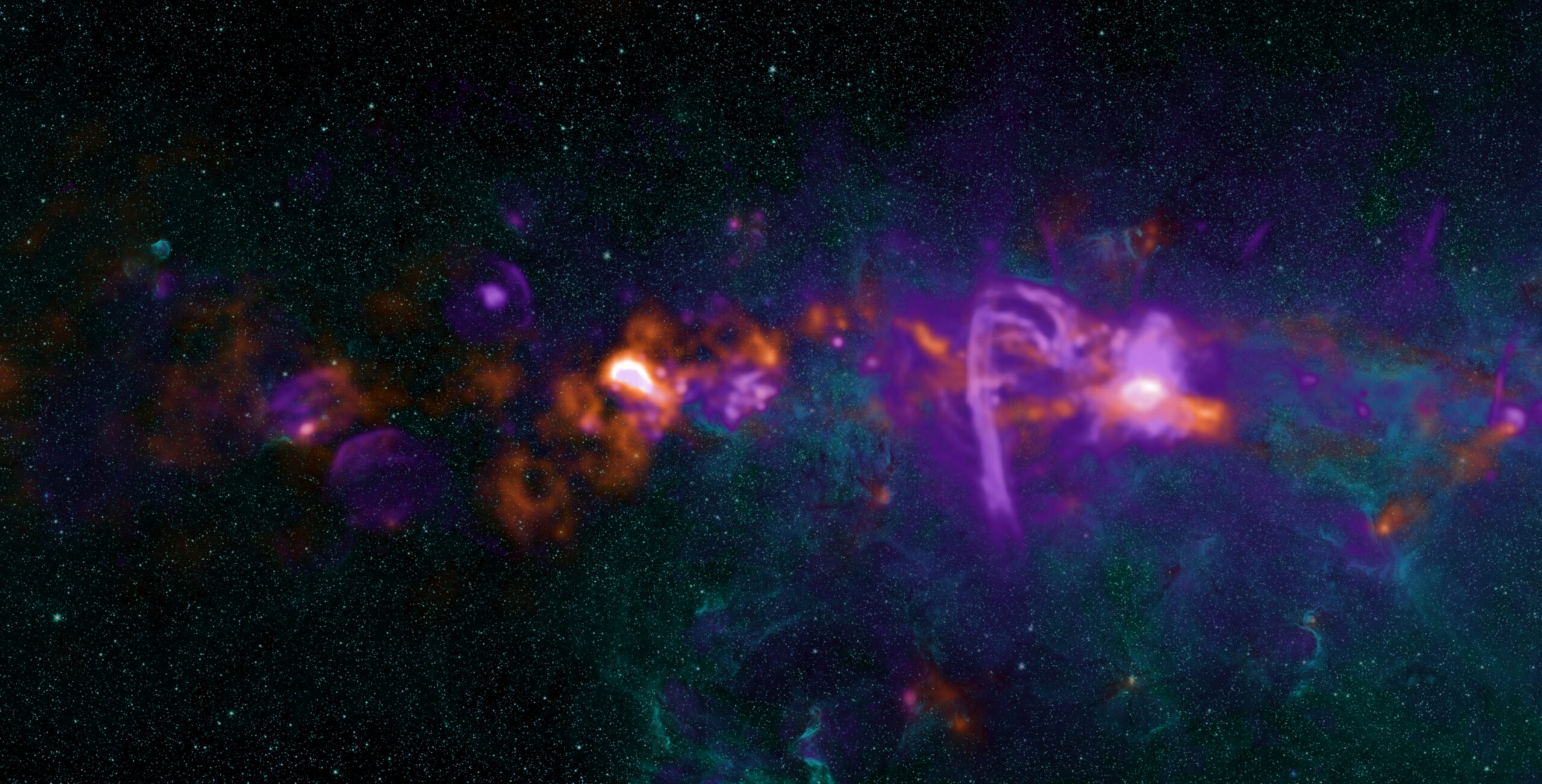
central molecular zone

The galactic center and the surrounding central molecular zone make up the most active star formation region in the Milky Way. [NRAO/AUI/NSF; CC BY 4.0]

Rojita Buddhacharya (Center for Astrophysics | Harvard & Smithsonian; Liverpool John Moores University) presented new results from the central molecular zone (CMZ), the dense gas reservoir at the center of our galaxy about 25,000 light-years from Earth. The CMZ is one of the most extreme environments we know of: gas there is roughly a hundred times denser, hotter, and more turbulent than what we see in nearby molecular clouds. Despite holding huge amounts of star-forming fuel, the CMZ forms stars at a surprisingly inefficient rate, and one of the puzzles is what conditions actually let any of that gas collapse into stars.

Buddhacharya mapped how gas transitions from highly turbulent, supersonic motion to calmer, subsonic motion across a region in the CMZ. This transition is well known in nearby clouds, where it usually precedes gravitational collapse, but it had never been clearly resolved in the CMZ before. Their team found a “calm island” of subsonic gas embedded in the otherwise turbulent sea. This is the first observation of its kind in the galactic center.

The Multi-Age Stellar Populations of Terzan 5 as Revealed by JWST

R. Michael Rich (University of California, Los Angeles) presented new JWST and Hubble Space Telescope observations of Terzan 5, an unusual stellar system near the center of the Milky Way that looks like a globular cluster but doesn’t act like one. Earlier work had already shown that Terzan 5 hosts at least two distinct stellar populations with very different ages and chemical abundances, which is unusual for a typical globular cluster.

Because Terzan 5 sits behind a thick screen of foreground stars and dust, separating real cluster members from contamination is one of the hardest parts of the analysis. The team combined JWST and Hubble imaging to measure stellar proper motions, then used a vector point diagram to isolate the stars that move together with the cluster. They identified two additional stellar populations beyond the two already known. Rich argued that Terzan 5 may be a “fossil fragment,” possibly the leftover core of a small galaxy or early bulge structure that was accreted long ago.

Sub-Day Periodic Variability of Two Central Stars of Planetary Nebulae

Gaoyang Du (Dalian University of Technology) reported the discovery of new short-period signals in the central stars of two planetary nebulae. These central stars are the hot, exposed cores left behind by Sun-like stars at the end of their lives, and finding rapid brightness variations in them tells us about their interior structure and pulsation physics.

Short-period signals well under a day are very hard to recover from the ground because Earth’s rotation introduces strong one-day aliasing, so the team turned to the Transiting Exoplanet Survey Satellite, which observes continuously from space. Using a neural-network pipeline designed to handle the crowded, contaminated backgrounds these stars sit in, they recovered the previously known variability in NGC 1501 and detected a new signal at roughly half an hour. Follow-up spectroscopy will be needed to pin down whether the signals come from pulsations, rotation, or something else, but the result opens a new window on the rapid variability of dying-star cores.

Artificial Light at Night Significantly Degrades the Value of Public Lands

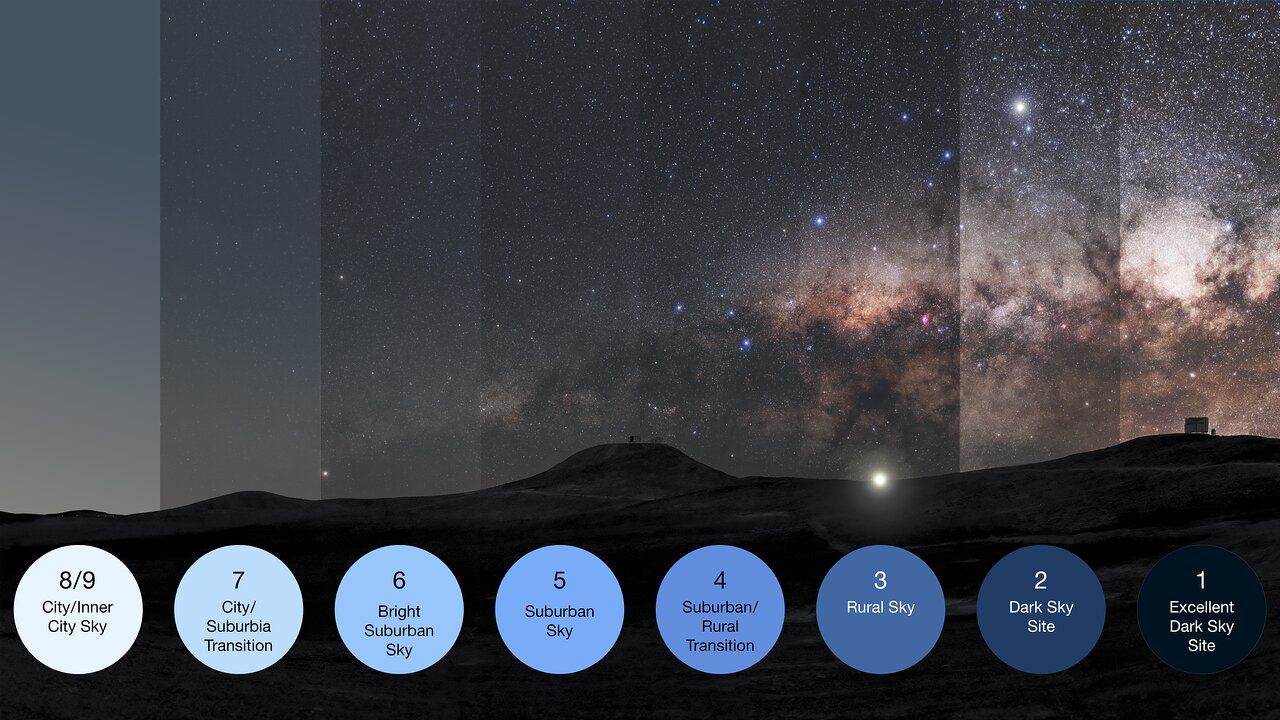
Jordan Smith (Utah State University) closed the press conference with a very different kind of measurement: the economic value of dark night skies. While astronomers usually treat light pollution as an observing problem, Smith and his collaborators are asking what the public is actually losing and what people would pay to keep dark skies on public lands. The team surveyed 634 visitors across International Dark Sky-certified parks, asking detailed questions about visitation behavior, motivations, and willingness to pay. Combining those surveys with satellite-based sky-brightness data, they estimated how the actual darkness of a site translates into the value visitors place on a trip. Based on the survey results, they found that visitors were willing to pay $45 more per visit to go to a park with skies one level darker on the Bortle scale. That sounds small per visitor, but scaled across all visits to all dark-sky public lands, it represents a very large economic value tied to a public good that current policy frameworks rarely account for.

illustration of the Bortle scale

An illustration of the Bortle scale, which quantifies the degree of light pollution at a given location. [ESO/P. Horálek, M. Wallner; CC BY 4.0]

Return to Table of Contents.

High Energy Astrophysics Division Early Career Prize Lecture: Carolyn Kierans, Developing Next-Generation MeV Telescopes (by Niloofar Sharei)

Carolyn Kierans (NASA Goddard Space Flight Center) was awarded the AAS High Energy Astrophysics Division Early Career Prize for her work on developing the next generation of megaelectronvolt (MeV) gamma-ray telescopes. Her talk laid out why the MeV band is so valuable (it contains nuclear emission lines like the 511 keV positron-annihilation line that traces high-energy processes in our galaxy) and why it has been so technologically difficult to observe well, since photons at these energies do not focus easily and the dominant interaction in the detector is Compton scattering. She walked through her work using balloon-borne Compton telescopes to mature the technology, the tools her team has developed in recent years to improve event reconstruction, and the broader roadmap for the next generation of MeV instruments.

Read Astrobites’s interview with Carolyn Kierans.

Return to Table of Contents.


Press Conference: Fire and Ice in Planetary Systems Near and Far (Briefing video) (by Kerry Hensley)

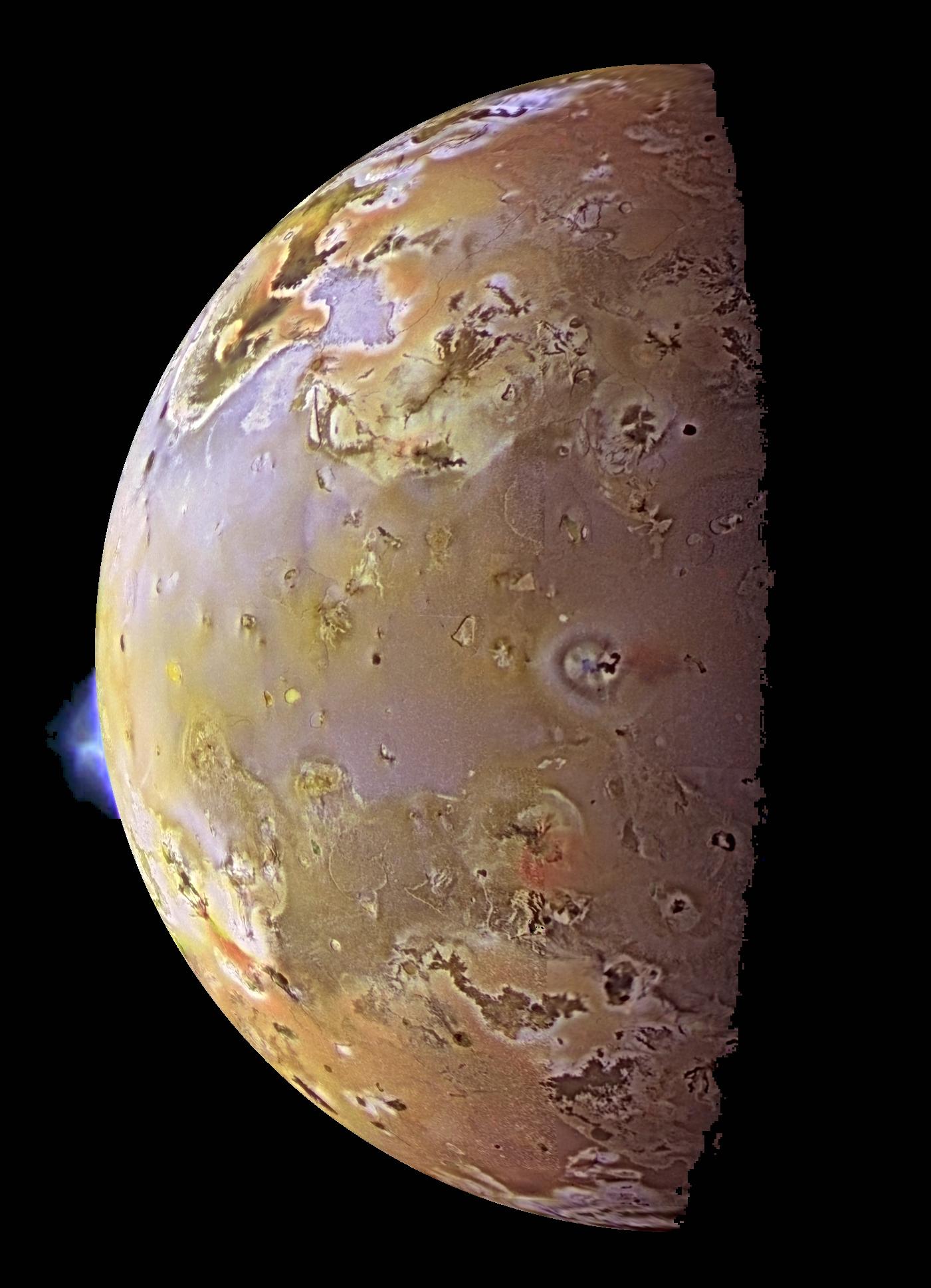
volcanic plume on Io

An image from the Galileo spacecraft of a volcanic plume on Jupiter’s moon Io. [NASA/JPL/University of Arizona]

The afternoon press conference was convened by Astrobites’s own Niloofar Sharei, this meeting’s Astrobites Media Intern. First up in the parade of planetary presentations was Neal Turner (NASA’s Jet Propulsion Laboratory/Caltech). Turner’s focus was Io, a moon of Jupiter and the most volcanically active body in the solar system. Turner’s team put forward a new claim: that the long-lived volcanoes that speckle Io’s surface spew out volcanic ash in their plumes, producing enough of this material to rapidly erase impact craters.

The team modeled Io’s plumes in order to explain the moon’s lack of impact craters, understand how certain plumes have persisted on Io for more than 45 years, and motivate a possible mission concept that includes a plume flythrough and sample return. They modeled the formation of ash as magma rises in a volcanic vent as well as the trajectory of the ash once it’s ejected into the plume, aiming to 1) match the plume observations from the Galileo spacecraft and 2) understand how an ash-filled plume might look different from one filled only with sulfur dioxide. While Turner found that Galileo data couldn’t discern between the two scenarios, ash makes a dramatic difference at the sub-millimeter wavelengths accessible to the Atacama Large Millimeter/submillimeter Array, which the team hopes to use to test this prediction. Finally, returning to the development of the mission concept, Turner proposed using a probe to first fly through the shadow of a plume to assess the particle size before sending the spacecraft through to collect a sample.

Up next, Tunhui Xie (University of California, Los Angeles) turned to Io’s neighbor, Europa. Europa and the other large icy moons of Jupiter are of interest to researchers because they might have subsurface oceans. Observations of Europa from ~30 years ago show that the moon has strange radar properties: its radar albedo is large, and the return signal retains the strong circular polarization of the outgoing signal.

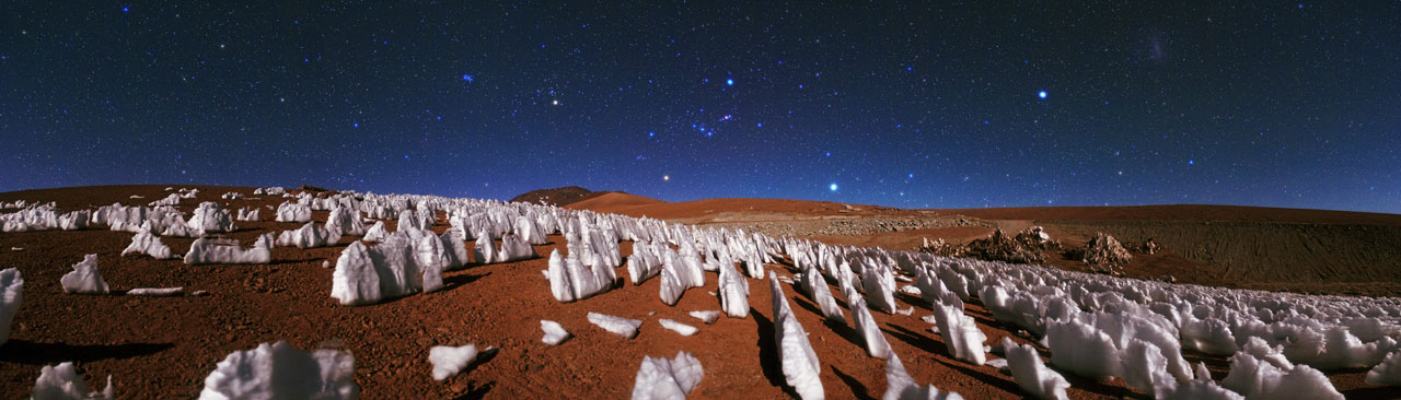
To investigate the moon’s radar weirdness further, Xie’s team observed Europa from 2011 to 2024 and showed that the moon’s albedo (fraction of light reflected from its surface) is roughly constant with longitude. There is some evidence of differences between Europa’s hemispheres, which could be a sign of spiky ice structures called penitentes protruding from the frosty surface; Europa’s trailing hemisphere might be subjected to more particles from Jupiter’s magnetosphere, which could suppress the growth of penitentes in that region and cause a difference in the albedo. Xie also addressed the polarization behavior of the radar signal, showing that this is likely due to the coherent backscatter opposition effect. Finally, Xie showed how observations helped to place an upper bound of 32 meters for the penetration depth of X-band radar photons into Europa’s icy shell.

penitentes

Penitentes in the Atacama Desert. [ESO/B. Tafreshi (twanight.org); CC BY 4.0]

Bryce Bolin (Eureka Scientific) reported on the third known visitor from another star system: 3I/ATLAS. Using the Multi-Object Spectrograph for Infrared Exploration on the Keck I telescope, Bolin’s team obtained some of the first infrared images of the interstellar visitor and detected its fuzzy coma — the cloud of gas and dust that surrounds the solid body of the comet — shortly after its discovery in July 2025. In August, observations revealed that the comet had started to grow a tail. As the team monitored 3I/ATLAS during its journey through our solar system, they saw significant changes. The comet was initially very red, likely due to space weathering from the galactic environment, but it became greener as the comet became active and refreshed its surface.

In some of the earliest spectroscopy taken by a large-aperture telescope, Bolin’s team found cometary volatiles like CN, but not C2 or C3, which are common in comets, giving them a green color. These missing species emerged a couple of months later, which coincided with the comet taking on a greener appearance. As the comet retreated from its encounter with the Sun, these emission features faded. This presentation by Bolin showed how early and continuing monitoring of an interstellar object by a large-aperture telescope can reveal how these objects are affected by their journeys through our solar system.

Moving out of the solar system entirely, Tiffany Kataria (NASA JPL/Caltech) turned the discussion toward exoplanets. Kataria discussed HD 80606b, a 4.1-Jupiter-mass planet on an extremely eccentric (e = 0.93) orbit with a period of 111 days around a solar-type star. Kataria used JWST to observe HD 80606b’s phase curve, which revealed different parts of the planet as it travels along its orbit. Each time the planet makes its extremely close approach to its host star, it gets “flash roasted” and experiences a rapid increase in temperature. This rapid heating event is complex, depending on factors like the planet’s atmospheric chemistry and winds. The JWST data revealed that HD 80606b’s temperature skyrockets an incredible 1,100℉ over the course of its orbit. There’s still much more to learn from the rich spectroscopic dataset from JWST, so keep an eye out for more findings about this flash-roasted exoplanet in the future!

Finally, Aurora Kesseli (IPAC/Caltech) discussed another toasty exoplanet called CoRoT-2b, which is a hot Jupiter on a 1.7-day orbit around its star. Because hot Jupiters orbit their hosts so closely, astronomers expect all of these extreme exoplanets to be tidally locked, with one side of the planet perpetually facing the star and the other side in perpetual darkness. However, CoRoT-2b might be breaking that trend. In 2018, researchers reported that CoRoT-2b had winds that blew in the opposite direction from all other known hot Jupiters. They drew this conclusion from the location of the hottest point on CoRoT-2b, which appeared just after the planet ducked behind its star, rather than just before — unlike all other hot Jupiters studied so far. At the time, researchers hypothesized that the unusual location of the hotspot was due to clouds on one side of the planet, a magnetically induced westward wind, or a lack of tidal locking.

Using new data from the Very Large Telescope and Gemini South, Kesseli found that the planet’s strange properties can be explained best by a lack of tidal locking. CoRoT-2b appears to rotate at 2.24 km/s — far slower than the 4.37 km/s expected if the planet were tidally locked. There are no theories yet that explain why CoRoT-2b wouldn’t be tidally locked, so it remains a mystery for now!

Return to Table of Contents.


Solar Physics Division George Ellery Hale Prize Lecture: Yi-Ming Wang, The Sun as a Laboratory for Astrophysical Magnetic Fields (by Kerry Hensley)

Yi-Ming Wang (Naval Research Laboratory) gave the AAS Solar Physics Division’s George Ellery Hale Prize Lecture for “sustained, foundational contributions to understanding solar magnetism, the solar cycle, and the solar wind.” Wang is perhaps most known for the Wang–Sheeley–Arge solar wind model, which is widely used in space weather forecasting.

Wang began by musing on how his winding career path brought him to solar physics. Initially a theorist who modeled neutron stars, Wang was later hired to do radio astronomy but arrived for the position later than expected, so he was roped into working on solar physics instead — where he learned many things about magnetic fields that he wished he’d known when working on neutron stars!

extreme-ultraviolet image of the Sun

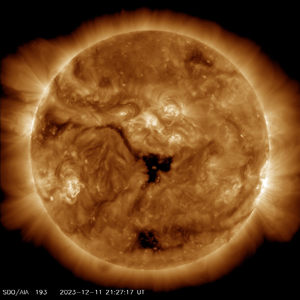
This 19.3-nanometer image, taken by the Solar Dynamics Observatory on 11 December 2023, shows at the center of the Sun’s disk the remnant of a large coronal hole. [NASA/SDO and the AIA, EVE, and HMI science teams]

In this talk, Wang gave an overview of three aspects of the Sun related to its magnetic field: quasi-rigid rotation of coronal holes, the source of coronal heating, and the speed of the solar wind. First up, coronal holes: these are dark areas in the solar corona where magnetic field lines stream out into space, which solar physicists call “open” field lines. (“Closed” field lines curve back to the solar surface.) Wang described how we know that coronal holes are regions of open field lines by extrapolating the photospheric magnetic field. (The photosphere is the visible “surface” of the Sun.) Because coronal holes rotate quasi-rigidly (compared to the photosphere, which rotates differentially), magnetic field lines must be continually converted from closed to open and vice versa at the boundaries of these holes.

Next, Wang discussed the source of coronal heating. The solar corona is famously extremely hot, running at a few million degrees compared to the ~6000K solar photosphere. For decades, the Parker nanoflare model has been the leading explanation for how the corona gets so hot. In this model, the places where coronal loops touch down in the solar photosphere are continually wiggled around by random motions of the photosphere, which tangles up the magnetic field lines in the coronal loop. When the current sheets in this system dissipate, the corona is heated. Instead, Wang favors an observationally based model in which the heating comes from magnetic reconnection with underlying small-scale fields.

Finally, Wang briefly touched on the connection between the Sun’s magnetic field and the speed of the solar wind. The solar wind has been measured at Earth since the 1960s, and these measurements have shown that the mass and energy flux density of the solar wind scales with the strength of the footprint magnetic field strength, but the observed solar wind speed is independent of the footprint field strength. Instead, the speed scales inversely with the rate of magnetic flux-tube expansion in the corona. Thus, the solar wind speed at Earth can be calculated from the rate of flux-tube expansion along open magnetic field lines using maps of the photospheric magnetic field.

In the end, Wang’s work on the solar magnetic field did connect back to his earlier work in high-energy astrophysics, with relevance to period changes in binary pulsar systems and other areas. Magnetic fields really do connect all parts of astrophysics!

Read Astrobites’s interview with Yi-Ming Wang.

Return to Table of Contents.


Plenary Lecture: David Jewitt, The Interstellar Interlopers (by Niloofar Sharei)

David Jewitt focused his plenary talk on a rare kind of small body: the three confirmed interstellar objects that have passed through the solar system so far. He opened with the Oort cloud as a framing device. Comets in the Oort cloud did not form there — they formed near the giant planets and were scattered out by gravitational interactions. The same process leaks comets to interstellar space very efficiently: only about 1–10% are trapped into a star’s own Oort cloud. Across the galaxy, that implies a free-floating population on the order of 1024–1025 objects. Seeing some of them pass through our solar system is exactly what we should expect.

artist's impression of Oumuamua

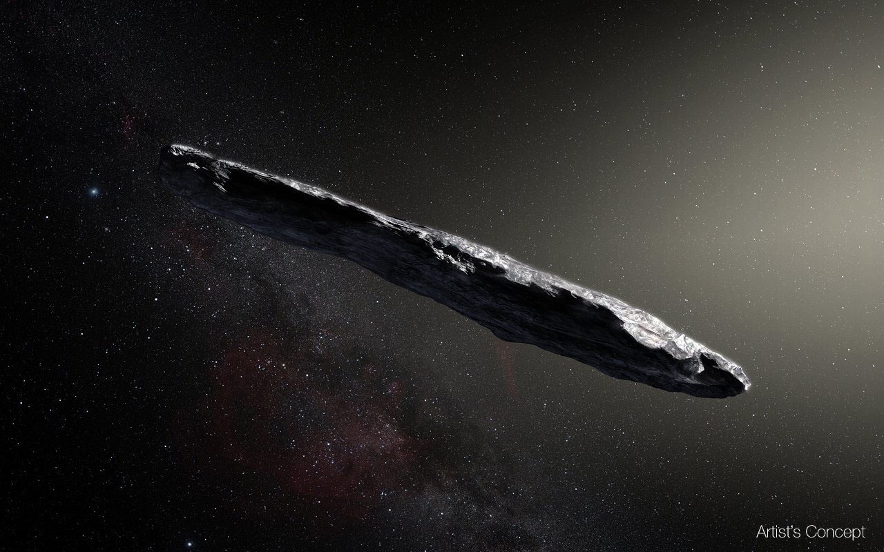
Artist’s impression of the first known interstellar object to visit our solar system. ʻOumuamua. [ESO/M. Kornmesser; CC BY 4.0]

The bulk of the talk walked through the three known interlopers. ʻOumuamua (1I/2017 U1) is the strangest: a tiny inert body about 80 meters across, with an extreme light curve consistent with either a 6:1 elongated shape or a flattened disk, and a non-gravitational acceleration of about 0.1% of solar gravity despite no detectable outgassing. Jewitt walked through the proposed explanations: exotic ices, ultra-low-density fluffballs, and sail-like sheets, and showed why each runs into a physical problem. 2I/Borisov (2019), by contrast, looks like a perfectly normal comet, with a ~400–500-meter nucleus, a coma, a tail, and a solar-system-like composition. 3I/ATLAS is the largest at roughly a kilometer, and JWST infrared spectroscopy has revealed CO2 emission about an order of magnitude richer than typical solar system comets. This is the first detailed look at the volatile inventory of an interstellar visitor.

Jewitt then turned to what the three objects tell us as a population. The strongest constraint comes from ʻOumuamua, precisely because its discovery was such a near miss: catching one in that brief visibility window implies roughly 1,000 similar objects crossing the solar system per year. The three objects look very different in size, activity, and composition, which is consistent with sampling a broad galactic population, and their velocity dispersion lines up with the disk-heating picture, in which older galactic populations are kinematically hotter. The leading origin story is the same one he set up at the start: scattering from the protoplanetary disks of giant planets around other stars.

Read Astrobites’s interview with David Jewitt.

Return to Table of Contents.

The post AAS 248: Day 2 appeared first on AAS Nova.

  •  

AAS 248: Day 1

Virgo Cluster

Editor’s Note: This week we’re at the 248th AAS meeting in Pasadena, CA. Along with a team of authors from Astrobites, we will be writing updates on selected events at the meeting and posting each day. Follow along here or at astrobites.com for daily summaries, or follow @astrobites.bsky.social on Bluesky for more coverage. The usual posting schedule for AAS Nova will resume on 22 June.

Table of Contents:


Fred Kavli Plenary Lecture: Richard Teague, Revealing the Dynamics of Planet Formation (by Lexi Gault)

Richard Teague (Massachusetts Institute of Technology) gave the Fred Kavli Plenary Lecture on his groundbreaking work in the dynamics of planet formation. The study of planet formation, as Teague introduced, has advanced significantly in the last two decades with the discovery of thousands of exoplanets and the launch of cutting-edge instruments. While planets are found everywhere orbiting a wide variety of stars, not all planetary systems look the same. Our solar system looks very different from other exoplanetary systems, challenging our understanding of planet formation and requiring us to build a picture that works across the board.

Where do we look to build a better understanding of planet formation? Planets are inherently the byproduct of star formation, forming in protoplanetary disks around new stars. These disks are filled with gas and dust, concentrating mass into rings that then eventually form planets. Exactly how this process proceeds is variable, and the resulting planetary system depends on how the material in the protoplanetary disk mixes and combines into planets. Teague compared planets to bread: we know the simple list of ingredients that it takes to make them, but what you end up with depends on how you bring those same ingredients together. We need to study what is happening in the planetary mixing bowls to understand how planets form.

exoALMA disks

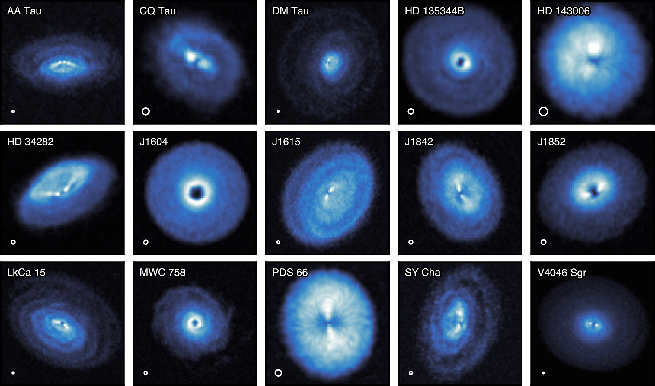
The full exoALMA sample. All 15 disks show evidence of substructure in their gas emission. [Teague et al. 2025]

Leveraging the high spatial and spectral resolution of the Atacama Large Millimeter/submillimeter Array (ALMA), Teague and collaborators have developed exoALMA, a planet-hunting campaign focusing on the still-forming planets of protoplanetary disks. This project has focused on 15 sources, obtaining and analyzing high-resolution observations to explore the kinematics, 3D velocity structures, and mass distributions within these protoplanetary disks.

The first science results from exoALMA have started to reveal that the planet formation process is highly dynamical — precise kinematic measurements uncover dynamical perturbations within protoplanetary disks across their sample. These perturbations point to the impacts protoplanets have on disk kinematics and mass distributions as they continue to form, and the high resolution of ALMA observations unlocks the inner workings of protoplanetary disks.

Looking forward, Teague emphasized that the future is broad for planet formation science. The upcoming Wideband Sensitivity Upgrade on ALMA will enable even more detailed maps of protoplanetary disks, unlocking the mysteries of planet formation while it happens.

Return to Table of Contents.


Press Conference: The Science of Stellar Remnants (Briefing video) (by Lucas Brown)

In AAS 248’s very first press conference session, we heard from a variety of scientists and research teams on all sorts of stellar remnants: white dwarfs, supernovae, pulsars, and beyond. Basically, if it came from a dying star, it was fair game for this session.

Boron and Beryllium as Unlikely Probes of Extrasolar Planets

First up was Ben Zuckerman (University of California, Los Angeles), who updated us on ongoing research into the presence of boron and beryllium in certain white dwarf systems. For some context, there exist many white dwarf systems in which a companion object — sometimes a planet — can have its material accreted onto the surface of the white dwarf due to tidal disruption during close approaches in its orbit. This deposition of material can then be detected via spectral signatures in observations of the white dwarf.

In 2021, evidence was first presented for two white dwarfs being “polluted” with trace amounts of beryllium, which is a particularly rare element, cosmically speaking. This raises the question of how so much beryllium ended up in these systems. In the hunt for answers, however, another mystery has emerged: missing boron. As Zuckerman went on to describe, boron was also recently discovered in some of these white dwarf systems, but at an abundance roughly equal to that of the beryllium. This is despite boron being about a hundred times more common in the universe, further muddying the waters of what exactly is causing such a strange pattern of heavy metals in these systems. Work remains ongoing to find a physical model that can reconcile these observations.

White Dwarf Kicks via Episodic Mass Ejection from Red Giant Stars

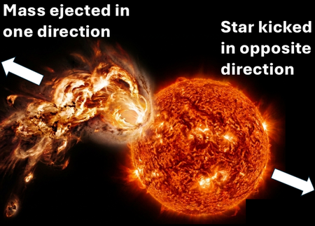
Image showing a star undergoing a massive coronal ejection event. Text superimposed on the image indicates that the mass being ejected in one direction pushes the star in the opposite direction.

In the model explored by Jim Fuller and collaborators, repeated mass-ejection events can cause red giant stars to be “kicked” up to a relatively high velocity before they collapse to form white dwarfs, explaining the high velocities many white dwarfs are observed to have. [Jim Fuller]

Next we heard from Jim Fuller (Caltech). Fuller filled us in on some recent studies aiming to explain why white dwarfs often obtain such high velocities when formed. Just like our own Sun occasionally ejects plumes of plasma from its surface, the red giant stars that eventually form white dwarfs are expected to periodically undergo mass-ejection events. But unlike with our own Sun, these ejections can shear off a significant amount of the star’s total mass — up to ~0.01% per ejection. Each time such an ejection occurs, Newton’s 3rd law ensures that the star itself will also receive a random velocity boost in the opposite direction. Over many thousands of ejections, assuming they occur randomly in all directions, this can significantly “kick” a meandering red giant up to speeds exceeding half a kilometer per second. Once such a star collapses to form a remnant white dwarf, the white dwarf will have this excess velocity too.

Additionally, this random ejection process predicts that red giants in binary systems will experience a sort of “random walk” in their orbital parameters, not just their overall velocity. This can lead to the complete dissociation of binaries, or to the direct collision of a red giant with its companion — leading to predictions about how many widely spaced white dwarf binary systems should exist. | Press release

Probing Intrabinary Material in a New Spider Millisecond Pulsar

Rebecca Kyer (Michigan State University) gave an update on research into so-called “spider” millisecond pulsars. These rapidly rotating neutron stars are a sub-class of pulsar characterized by their very high spin rate and the presence of a companion from which the pulsar is accreting material. Such systems are further sub-classified as either “Black Widows,” which have very low-mass companions (~3% solar mass), “Redbacks,” which have larger companions at ~10-80% solar mass, and “Huntsmans,” which have more massive red-giant companions. These Huntsman pulsars are the newest category, with only two known cases — until now!

Kyer presented evidence collected by their team that may indicate the discovery of a third Huntsman pulsar. The evidence involves radial velocity measurements of the companion star, which shows an orbital period of 3.64 days and variable H-alpha emission. In these systems, the radio emission typically associated with the pulsar can be blocked from our view for unpredictable amounts of time due to clouds of hot gas and dust that emerges from the complex interaction between the pulsar and red giant winds. Despite this, Kyer hopes that with enough targeted observations with the Green Bank Telescope, a radio signal will eventually be detected, confirming the pulsar’s presence.

Image of galaxy M83 in X-ray and optical light.

Image of Messier 83 in both X-ray and optical light. Prominent X-ray sources can be seen as small colorful blobs strewn throughout the galaxy. Some of these X-ray sources are supernova remnants, a subset of which have recently been found to show variability in their brightness. [X-ray: NASA/CXC/SAO; Optical: NASA/ESA/AURA/STScI, Hubble Heritage Team, W. Blair (STScI/Johns Hopkins University) and R. O’Connell (University of Virginia); Image Processing: NASA/CXC/SAO/A. Jubett, L. Frattare and P. Edmonds]

NASA’s Chandra Finds Unexpected Fireworks in Aftermath of Stellar Explosions

Finally, we heard from a team of three researchers — Andrea Prestwich (Catholic University of America / NASA Goddard SFC), Roy Kilgard (Wesleyan University), and Zoe Hoiland (Vassar College) — on an unexpected supernova discovery. Traditionally, supernovae are modeled as having a relatively constant or slightly decreasing luminosity, at least after their initial explosion. As the stellar material is blasted away from the progenitor’s core, it interacts with the surrounding interstellar medium and a blob of hot, shocked gas is left over. This blob will eventually cool and dim, but often over a long time period, leading to the aforementioned prediction of constant or slightly decreasing brightness.

However, in 14-year Chandra observations of a supernova remnant in Messier 83, Prestwich and her collaborators actually found significant X-ray variability, with the remnant occasionally even increasing in brightness. In a follow-up study, it was found that supernova remnants in Messier 51 likewise show this up-and-down variability. In contrast, an analysis of remnants in Messier 101 showed zero variable remnants. Notably, the former two galaxies are very actively star-forming, while the latter is not. Some possible theoretical models to explain this variability include the possibility of stellar material falling back on the compact object leftover by the supernova, creating an accretion disk that can generate variable emission. Alternatively, it has been proposed that there could be a neighboring star to the remnant object, forming an accreting X-ray binary system that could also induce variability. | Press release

Return to Table of Contents.


Plenary Lecture: Sanmi (Oluwasanmi) Koyejo, The Measurement Gap: What AI Can Get Wrong and Why Astronomers Are the Fix (by Lexi Gault)

Sanmi (Oluwasanmi) Koyejo, a professor of computer science at Stanford University, focused this plenary talk on the limitations of AI as it becomes more integrated with science and how astronomers can help solve these problems. Koyejo began by addressing the question of why an AI researcher is talking to astronomers. His research explores how to set AI standards and how to best assess the performance of an AI model, which becomes particularly important when these models are used to do science.

Evaluating the performance of an AI model relies on benchmarks, a fixed set of questions with known answers that are used to score the AI. These benchmarks are simple, reproducible, and comparable, but passing a benchmark does not equate to getting a meaningful scientific result. Benchmarks assume cheap checks, fast feedback, and fixed questions, but science is none of those things; answering astronomy questions relies on telescope time, and ground truth cannot be found quickly.

Much like telescopes, AI benchmarks are measuring instruments with noise that can compound. If you run an AI model many times, the goal is often convergence on an agreed-upon answer, but getting to an agreed-upon answer does not mean that the answer is correct. Koyejo’s recent research found that AI models more often agreed with each other than they did with the actual truth. This is made worse when AI is used to evaluate itself. For example, Koyejo notes the rising number of academic paper submissions due to AI-written papers greatly exceeds the capacity of human reviewers. If AI tools are used to evaluate AI-generated paper submissions, the AI will tend to favor AI-written materials, ignoring the actual scientific merit. Making evaluation of AI an AI problem compounds its failures, straying further from a correct answer.

This is where astronomers come in. Having the expert knowledge of what “correct” looks like, being able to judge which errors matter, access to expensive ground truth (telescope time), and a culture of blind analysis (not knowing exactly what the answer should be), astronomers are well equipped to build standards for AI evaluation. We can define what good AI is for astronomy and use our expertise to help build the standards. Koyejo left the audience with the charge to engage with AI (engagement does not mean endorsement), so that astronomers can help set the standards for appropriate AI use in science.

Read Astrobites’s interview with Sanmi Koyejo.

Return to Table of Contents.


Press Conference: Variable, Windy, and Disruptive: The Behavior of Supermassive Black Holes (Briefing video) (by Niloofar Sharei)

This press conference focused on what supermassive black holes do to the world around them, from relativistic jets of the most famous black hole, to the multi-phase winds launched from active galactic nuclei, to temperature-shifting coronae, and even the radio burps that are produced years after a black hole tears apart stars.

Chandra Tracks the Evolving Jet from Messier 87’s Black Hole: 

Camille Poitras (Laval University) presented the largest Chandra X-ray movie of jet evolution in the famous supermassive black hole Messier 87 (M87). M87 has been studied across the electromagnetic spectrum, but X-ray observations of its jet have always suffered from blur because high-energy photons are hard to focus. Using improved Chandra calibrations and deconvolution techniques, the team produced a 13-year X-ray movie of M87’s jet from 2012 to 2025. Tracking a bright knot within the jet, Poitras’s team saw it split into two components in 2023, with one component moving at an apparent five times the speed of light (which is a known illusion called superluminal motion). That allowed the team to look into where and how the particles are being accelerated to extreme energies along the jet. | Press release

Watching a Black Hole Wind Grow: Chandra and Hubble Reveal the Early Stages of Galaxy

Multi-wavelength images of two quasars

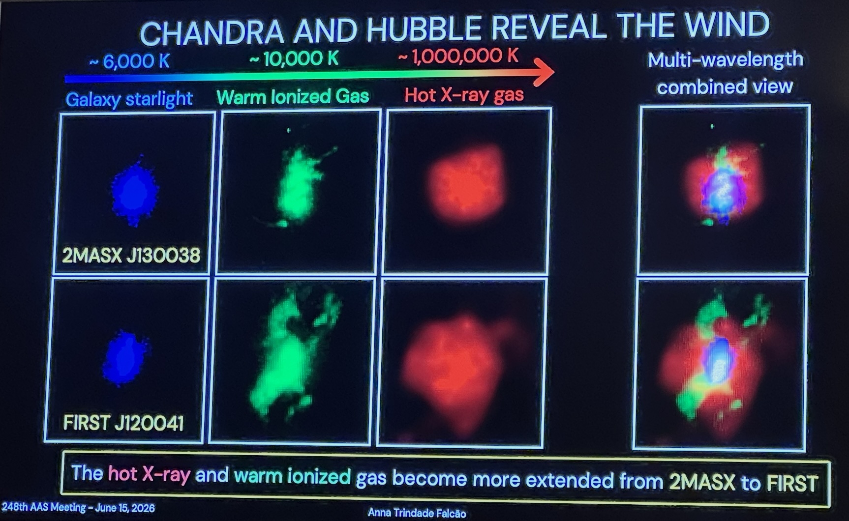
Multiwavelength images of two nearby quasars show that the hot X-ray (red) and warm ionized (green) gas are far more extended in the bottom system. Click to enlarge. [Anna Trindade Falcao]

Anna Trindade Falcao (NASA Goddard SFC) presented combined Chandra and Hubble observations that may capture a supermassive black hole wind in its earliest stages of growth. Active galactic nucleus (AGN) feedback is thought to happen, but how it begins remains poorly understood. Studying two nearby quasars in which Chandra (tracing hot X-ray wind) and Hubble (tracing warm ionized gas) data are aligned, the team found that the hot and warm phases extend together and not independently. This would suggest a single multi-phase outflow. Their team proposed a four-stage sequence for AGN feedback and also argued that their two systems capture the earliest stages of that process.
three black hole wind types at increasing distances

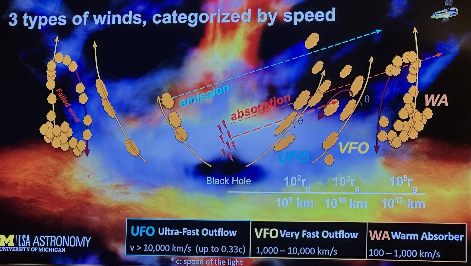
The three types of wind launched from an accreting supermassive black hole. Click to enlarge. [Xin Xiang]

XRISM Reveals Changing Accretion-Driven Winds in a Nearby Active Galaxy:

Xin Xiang (University of Michigan) presented the most detailed X-ray portrait of the winds flowing out of NGC 4151, an active galaxy roughly 16 million light-years away with a 30-million-solar-mass black hole. Every major X-ray observatory has observed this galaxy before, but earlier instruments could not separate its multiple wind components. With the high-resolution X-Ray Imaging and Spectroscopy Mission (XRISM) spectrometer, Xiang resolved three wind populations by velocity: warm absorbers (100–1,000 km/s), very fast outflows (1,000–10,000 km/s), and ultra-fast outflows (over 10,000 km/s). Across 14 XRISM observations over a year, they found that the fast winds turn on three hours after each bright X-ray flare, matching the predicted timescale for magnetically driven wind. | Press release

NuSTAR Reveals a Significantly Variable Active Galactic Nucleus Corona

Xiurui Zhao (Caltech) presented the first observational evidence of significant temperature variation in the corona of an AGN. The corona produces about 90% of all X-ray photons from an AGN, but its temperature can only be measured with X-ray missions sensitive to high-energy spectral curvature like NASA’s NuSTAR. They compared NuSTAR’s observations across multiple years and found that despite having the same luminosity in 2015 and 2024, the 2024 corona was significantly cooler than the 2015 corona. In follow-up observations in 2025, it was back at its earlier temperature. This is the first clear observation of coronal temperature variability in an AGN. | Press release

New Surprises from Radio Observations of Tidal Disruption Event Outflows

Kate Alexander (University of Arizona) presented new radio observations of tidal disruption events (TDEs). TDEs occur roughly once every 100,000 years in a given galaxy. It happens when a star drifts too close to the black hole, is stretched and squeezed into a long stream of debris (a process astronomers call spaghettification) and some of that debris falls onto the black hole while the rest is thrown outward and lights up in radio. Alexander and her team used six years of Very Large Array monitoring of several dozen nearby TDEs. They found that many TDEs unexpectedly turn on in the radio years after the original event, even long after their optical light has faded. Their team combined radio data with X-ray and optical accretion-rate measurements and found that these late-time radio flares appear when the black hole is eating either very quickly or very slowly, but not at moderate rates! This pattern matched what is seen in stellar-mass black holes and this suggests that accretion physics may operate similarly across many orders of magnitude in black hole mass. | Press release

Return to Table of Contents.


Plenary Lecture: Mario Jurić, Early Results from the Rubin Observatory: Mapping the Solar System and Beyond (by Kerry Hensley)

Mario Jurić (University of Washington; PI of the University of Washington Rubin operations element) began by remarking on how our collective concept of what an astronomer is has been transformed over the past 25 years. While a Google image search for “astronomer” yields an array of people pointing small telescopes at the night sky, today’s version of professional astronomy looks quite different: huge telescopes with enormous cameras covering vast swaths of the sky, with analysis aided by software and data deposited in massive databases.

This rapid transition was first spurred by enterprises like the Sloan Digital Sky Survey, which collected 20 terabytes of raw data from 1.2 billion observations. Now, digital sky surveys are common, and they’re becoming ever larger. The next massive digital sky survey will be the Legacy Survey of Space and Time from the NSF–DOE Vera C. Rubin Observatory — an observatory that can “download the universe” and is poised to transform our understanding of everything from asteroids to dark energy.

Rubin released its first images on 23 June 2025, and among these stunning images is a broad view that contains thousands of galaxies in the Virgo cluster, a golden tangle of four colliding galaxies, a nearby galaxy cluster, a distant galaxy cluster, and a handful of nearby spiral galaxies bursting with star formation. As fantastic as this image is, Jurić emphasized that it’s just one still image in a movie: as Rubin returns to the same fields of view time and time again, it’ll spot things that change brightness (like variable stars and transients) and things that move (like asteroids).

Jurić highlighted four areas in which Rubin has already contributed greatly, focusing on discoveries within our solar system:

    1. Asteroid variability: Rubin has already collected hundreds of thousands of observations of asteroids, resulting in the discovery of extremely fast rotators like 2025 MN45, which must have an extremely high tensile strength not to fly apart.
    2. Observations of interstellar object 3I/ATLAS: During the observatory’s commissioning survey, the Rubin team realized that they had observed 3I/ATLAS before it was discovered — but in observations that were technically under embargo. Recognizing the high impact of the data, the team found a way to share their findings, leading the 150-person collaboration to write a paper on their findings in a mere three days.
    3. High-precision asteroid photometry: While analyzing the commissioning data, the Rubin team discovered systematic offsets in the positions of asteroids — but no other types of objects. They found that this effect varied across the sky and was worse in the south. They eventually discovered that because most asteroids are observed from the north, that catalogs of asteroid orbits are systematically biased at a level of 20-40 milliarcseconds. Luckily, Rubin will provide the much-needed southerly data necessary to clean up these catalogs within about a year.
    4. Outer solar system studies: Researchers discovered 380 new trans-Neptunian objects in Rubin’s commissioning data. (Compare that to just 5,000 known trans-Neptunian objects in total!) In the time since the commissioning data were collected, hundreds more candidate objects were discovered.

With such enormous data yields from Rubin, how do we efficiently turn data into science? Jurić outlined strategies for handling massive datasets using well-crafted data formats, computing tools, and AI. In particular, Jurić highlighted the Astronomical Catalog Inference Driver, or ACID, which he built in four weeks on his phone using Claude. The tool is comparable to “a product developed in >3 years by extremely capable human professionals” and can rapidly handle immense data tables, showing how AI can accelerate the development of tools to handle tomorrow’s datasets.

Read Astrobites’s interview with Mario Jurić.

Return to Table of Contents.


Plenary Lecture: Esra Bulbul, Cosmology and Baryons Across Scales: Probing Halo Mass Function to Cosmic Filaments with eROSITA (by Lexi Gault)

Esra Bulbul (Max Planck Institute for Extraterrestrial Physics) began her plenary talk at the beginning of time — the Big Bang marked the start of the universe, and from there we attempt to constrain cosmological parameters in order to understand how the universe was born and how it has evolved. Bulbul notes that a lot of work has been done to constrain cosmology from the cosmic microwave background (CMB), and we must compare those early time measurements to those from later times to build a full picture. In cosmology, tensions have arisen between early-time and late-time probes. CMB measurements of the Hubble constant and S8, the “clumpiness” parameter of the universe, do not agree with late time probes that find that the universe is accelerating faster with smaller fluctuations than the CMB predictions. How do we work toward resolving this tension?

The extended ROentgen Survey with an Imaging Telescope Array (eROSITA) is a space telescope that has performed the first imaging all-sky survey in the medium X-ray range, seeking to map the large-scale structures of the universe to better constrain cosmological constants. eROSITA focuses on finding galaxy groups and clusters via the hot X-ray gas within and between them across the last 5-7 billion years of the universe. Since its launch in 2019, eROSITA has completed more than four full-sky surveys. Of the million X-ray sources detected by eROSITA, only 12,247 (1%) are galaxy clusters and groups.

From the observed X-ray emission from the galaxy clusters and groups, the eROSITA team has been able to measure the temperature of the intercluster medium within the sample. Working with weak gravitational lensing surveys, they have been able to measure the masses of the newly discovered clusters and groups. These measurements show that eROSITA has detected sources across three orders of magnitude in mass, reaching from the galaxy level to large-scale clusters.

The galaxy cluster and group observations allow them to constrain a few cosmological parameters including S8 (density fluctuations), Ωm (matter density), and w0 (dark energy). From the impressive eROSITA data, Bulbul showed that they could constrain S8 and Ωm to five times better precision than ever before! These late-time results are fully consistent with what has been measured from the early-time CMB measurements. Additionally, the dark energy measurements agree with what has been measured thus far from the Dark Energy Spectroscopic Instrument survey.

Bulbul then switched us from the exciting cosmological results to those regarding baryon detection. A striking result from eROSITA was the detection of hot gas well beyond what is typically considered the gravitational extent of a galaxy cluster — reaching out to 16 million light-years, often larger than the galaxy cluster itself. This underscores the importance of X-ray surveys in detecting the very extended gas encapsulating the largest-scale structures of the universe.

Looking forward, Bulbul discussed the future work planned for eROSITA. Transitioning now to working with the deepest data of the survey, the team expects to find about 40,000 galaxy clusters with about half of those being used for cosmology. They anticipate obtaining even higher precision on cosmological parameter measurements, comparable to that obtained from CMB observations. The work of eROSITA is revolutionizing cosmology at later times in the universe, and the future is exciting.

Read Astrobites’s interview with Esra Bulbul.

Return to Table of Contents.

The post AAS 248: Day 1 appeared first on AAS Nova.

  •  

Shining a Light on the Shadowy Movements in Saturn’s Rings

Editor’s Note: Astrobites is a graduate-student-run organization that digests astrophysical literature for undergraduate students. As part of the partnership between the AAS and astrobites, we occasionally repost astrobites content here at AAS Nova. We hope you enjoy this post from astrobites; the original can be viewed at astrobites.org.

Title: Dynamics of Planetary Rings Under Thermal Forces
Authors: Wen-Han Zhou et al.
First Author’s Institution: The University of Tokyo
Status: Published in ApJL

If you ask anyone what their favourite planet is, the answer you’ll most likely hear is Saturn. Why? Why else than the beautiful and intricate ring system surrounding the gas giant. The other gas and ice giants in our solar system — Jupiter, Uranus, and Neptune — have ring systems themselves but none quite as striking as Saturn’s. Would it surprise you to learn that astronomers’ best models have not yet totally explained why Saturn’s rings look the way they do?

In contrast, it may not surprise you to hear that people have been trying to explain the rings for as long as we have seen them with telescopes. We now know that planetary rings are collections of relatively small particles (think micrometre up to metre sized), most likely having once been the material of a larger body that was disrupted either by collisions or tidal forces. This material, due to the gravity of its local planet, is sculpted into a flat disc where more subtle interactions then lead to substructure forming within the disc such as gaps and ringlets. Many of these substructures are explained by well-understood physics — for example gaps being carved by embedded moonlets or resonances sculpting ring edges — though there remain some outstanding problems in our understanding.

The authors of today’s article set their sights on the problematic inner edge of Saturn’s A ring (Figure 1). They describe some mechanisms — namely the collisions of micrometeoroids within the rings — by which a sharp ring edge can be maintained, but there exists a gap in the understanding of how such an edge can form in the first place. All hope is not lost, though, as today’s authors reintroduce a physical process they call the “eclipse–Yarkovsky” effect, which seems to explain these phenomena.

horizontally sliced Saturn's rings

Figure 1: A horizontally sliced image of Saturn’s rings shows the rich substructure and gaps within the various rings. Saturn, which is not shown here, would be to the left of the image. The authors of today’s article are particularly concerned with the bright and sharp inner (left side) edges of the A and B rings. Click to enlarge. [NASA/JPL/Space Science Institute]

Billions of Rocket-Powered Bumper Cars

The idea behind this process revolves entirely around light. When sunlight hits a particle within a planetary ring, non-absorbed sunlight imparts a little “bump” onto a particle, ever so slightly altering its trajectory. At the same time, some of the sunlight is absorbed into the particle, which heats it up; light is soon re-emitted via thermal radiation, which, again, can slightly change the trajectory of these tiny particles. From a point on the surface of each ring particle (see rightmost side of Figure 2), the photons from this thermal radiation are all emitted in random directions; however, across the whole surface of the particle there is a net force! These tiny particles are spinning, and so the side just near “sunset” is hottest and emitting the most thermal photons. In this way, the pressure from the sunlight plus the thermal radiation of each particle imparts a net torque on the ring itself which changes the angular momentum of the ring.

diagram showing sunlight falling on Saturn and the planet casting a shadow on its rings

Figure 2: Starlight is the main source of light onto the particles that make up a planetary ring (right panel) though reflected light from the planet’s surface hits it too. This light “heats up” the ring and forms an asymmetry as the ring is eclipsed by the planet, which produces a net force. [Zhou et al. 2026]

What we described just then is essentially solar radiation pressure plus the Yarkovsky effect. It turns out that the net force from this process typically averages out to zero as the ring particles orbit around the planet. This assumes, though, that the sunlight is constantly shining on the ring. Stunning imagery of Saturn tells us that this isn’t the case, so what happens when we take into account the shadow cast on the ring from the planet? Today’s authors find that the net effect induces a positive change in angular momentum of the ring particles, which they call the eclipse–Yarkovsky effect.

After today’s authors detailed all of the math involved in this process (and there is a lot), they put it into practice to try to help explain Saturn’s curious rings. Including the eclipse–Yarkovsky effect together with other known effects that drive ring evolution allowed them to reproduce the optical depth profile (how thick the ring looks) of Saturn’s A ring better than ever before (notably the sharp inner edge in Figure 3). On top of this, the effect provides another avenue for moonlet formation in the outer edges of ring systems as the positive torque from the effect drives material out toward and away from the Roche limit.

plot of optical thickness versus radius

Figure 3: The authors try to explain the current structure of Saturn’s A ring by initialising it with a Gaussian profile of optical thickness versus radius (black dot-dashed line) and evolving it for 81 million years under different effects. When viscous effects are included (blue dashed line), the ring spreads out, but it’s only when the eclipse–Yarkovsky (EY) effect is included (red line) that the model closely matches the observed data (grey line). [Zhou et al. 2026]

Undeniably useful for Saturn, the eclipse–Yarkovsky effect may also explain some other conundra in the solar system. Mars may have once had rings, which are thought to have eventually clumped together to form the inner moon Phobos. This idea is problematic, though, in that current models suggest there should still be some residual ring system around Mars even after Phobos formed. Enter the eclipse–Yarkovsky effect: being 100 times stronger for Mars than Saturn (due to its more intense incident sunlight), the effect may have driven out and dispersed that residual ring altogether. While the authors are currently looking into this possibility, the reintroduction of the eclipse–Yarkovsky effect has already shown great promise for our most beautiful ringed planetary neighbour.

Original astrobite edited by Wasi Naqvi.

About the author, Ryan White:

I am a first-year PhD student at Macquarie University in Australia, working mainly on binary/multiple systems with massive stars (Wolf–Rayets in particular!). Outside of study, I’m probably drinking coffee, baking, reading, or going for a run. You can also find me procrastinating on Bluesky @astroryan.bsky.social.

The post Shining a Light on the Shadowy Movements in Saturn’s Rings appeared first on AAS Nova.

  •  

The First Starspot Spectrum Revealed by JWST

M-dwarf star with starspots

Editor’s Note: Astrobites is a graduate-student-run organization that digests astrophysical literature for undergraduate students. As part of the partnership between the AAS and astrobites, we occasionally repost astrobites content here at AAS Nova. We hope you enjoy this post from astrobites; the original can be viewed at astrobites.org.

Title: A Panchromatic JWST Spectrum of a Giant Starspot on the Fully Convective M Dwarf TOI-3884
Authors: C. A. Murray et al.
First Author’s Institution: University of Colorado Boulder
Status: Published in ApJ

We often picture stars as smooth, glowing spheres, as if they’ve been run through an Instagram filter. But real stars have spots: cooler, darker regions on a star’s surface caused by strong magnetic fields.

Annoyingly, these spots can seriously interfere with how we study exoplanet atmospheres.

How to Probe a Planetary Atmosphere

Planetary atmospheres are often probed through transmission spectroscopy. When a planet transits its star, some starlight passes through the planet’s atmosphere before reaching us. We can distinguish the light that has passed through the planet’s atmosphere by comparing the star’s light in transit versus out of transit. In doing so, we can isolate the atmospheric spectrum and look for absorption features of species like water or oxygen.

Easy, right?

How Starspots Get in the Way

Things get more complicated once we stop thinking of the star as if it’s been smoothed out by an Instagram filter. Starspots are cooler than the surrounding stellar surface, which means they emit a different spectrum. They are also constantly changing: new spots can form, old ones can disappear, and the star’s rotation carries them in and out of view. This changes things.

First of all, your star’s spectrum changes over time, which could mean that the star’s spectrum out of transit is not the same as the star’s spectrum during transit. On the other hand, the planet may transit across a starspot instead of a “normal” stellar region. In this case, the light we measure during the transit is affected by the spot, and it is no longer accurate to directly compare it with the overall stellar light outside the transit.

Ultimately, absorption features that we thought were from the planetary atmosphere could actually be coming from starspot contamination instead.

Starspot Models: Our Solution?

To deal with this, astronomers build starspot models, where they vary the spots in terms of the following:

  • The surface covering fraction: this parameter tells us how much of the stellar surface is covered in spots
  • The temperature contrast: this parameter tells us how much cooler (in ratio) the spot is compared to the rest of the stellar surface, and by proxy how much dimmer

These models are promising, but how do we know that we have chosen the right parameters?

A Unique Laboratory: TOI-3884

The TOI-3884 system is a unique laboratory for testing our starspot models. As seen in Figure 1, it has very convenient starspot geometry, with a large starspot located close to its pole. On top of that, we observe this star almost completely pole-on, which means that we always see this starspot, no matter how much the star rotates. To top this all off, the star hosts a close-in planet, which orbits the star from pole to pole.

Illustration of the TOI-3884 system

Figure 1: Illustration of the TOI-3884 system. The pole (and rotation axis) of the star is indicated with a black “x,” indicating that we see the star almost pole-on. The polar starspot is indicated in grey, and the transiting planet TOI-3884b is indicated in black. Different dates are shown, illustrating how the system evolves over the span of a few weeks. [Adapted from Mori et al. 2025]

The planet transits the star, and as it does so, it always passes over the polar starspot. This gives us a rare opportunity to probe the spectrum of a starspot. Similar to how we can use normal in/out of transit observations to probe a planetary atmosphere, we can now compare the observations during/after a “starspot transit” to probe the starspot region. Today’s authors do exactly this using six different transit observations from JWST.

So… How Good Are Our Models?

From the JWST observations, the authors extract a starspot spectrum for the first time. Figure 2 shows this as the spot contrast (how much dimmer the spot is than the surrounding stellar surface) plotted across different wavelengths. To see how well our models are doing, they compare this observed spectrum to two commonly used starspot models. The difference between the data and the models (the residual) is plotted in the lower panel.

spectrum of TOI-3884’s starspot.

Figure 2: The spectrum of TOI-3884’s starspot. The y-axis in the upper panel, the spot contrast, indicates how much dimmer the starspot is compared to the “normal” stellar surface. Different observations taken with JWST are indicated in different colored crosses, and other previous observations are overplotted in various other shapes. Model starspot spectra are shown in dashed or dotted black lines. The residuals between the model spectra and the JWST observations are shown in the bottom panel. [Adapted from Murray et al. 2026]

At wavelengths longer than about 1 micron, in the near-infrared regime, things look good! The residuals stay small, meaning the models do a solid job reproducing the observations. But move left into shorter wavelengths, in the optical regime, and the agreement quickly falls apart. The residuals grow, and it becomes clear that the models are missing something.

There’s still work to be done before we can confidently probe planetary atmospheres at optical wavelengths without worrying about stellar contamination, and this observed starspot spectrum provides a unique benchmark to test future starspot models. For now, the near-infrared remains a safer and more reliable window for planet atmosphere studies.

Original astrobite edited by Natalie Price.

About the author, Elise Koo:

I’m a PhD student at the University of Amsterdam, working to detect magnetic interactions between stars and their planets using radio and spectroscopic observations. Outside of research, I like to try out a variety of sports.

The post The First Starspot Spectrum Revealed by JWST appeared first on AAS Nova.

  •  

Life on the (Red) Edge

Earth in visible and near-infrared light

Editor’s Note: Astrobites is a graduate-student-run organization that digests astrophysical literature for undergraduate students. As part of the partnership between the AAS and astrobites, we occasionally repost astrobites content here at AAS Nova. We hope you enjoy this post from astrobites; the original can be viewed at astrobites.org.

Title: Retrieving the Red Edge on Earth-Like Planets with Heterogeneous Clouds and Surfaces
Authors: Zachary Burr et al.
First Author’s Institution: Jet Propulsion Laboratory; ETH Zurich
Status: Published in ApJ

In the next 25 years, astronomers could find signs of life on other planets with the launch of the Habitable Worlds Observatory. Atmospheric signs of life, known as atmospheric biosignatures, are how astronomers currently search for life on other planets. Figure 1 shows examples of atmospheric biosignatures with pictures of each chemical’s origin on Earth. Before E.T. can phone home, though, we have to understand what chemicals make up a planet’s atmosphere. To do this, astronomers can use spectroscopy to observe a planet’s atmosphere in different wavelengths and measure the types and quantities of chemicals present.
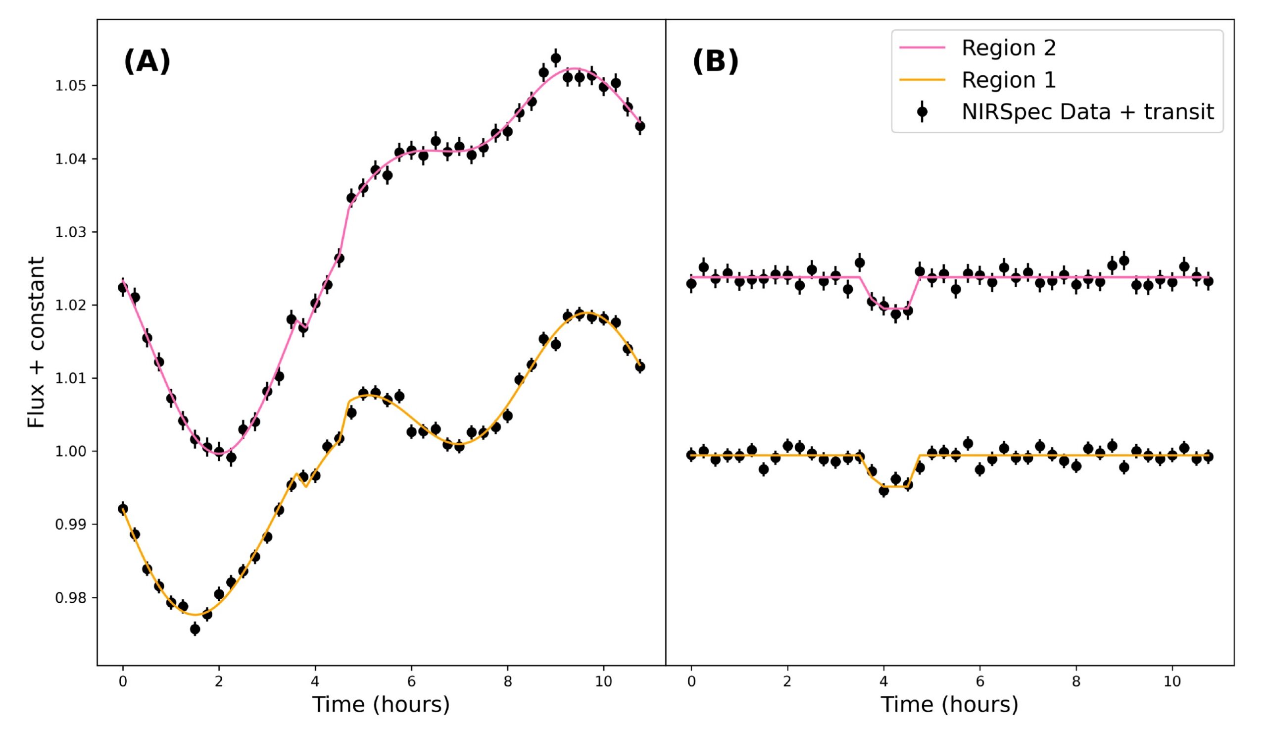
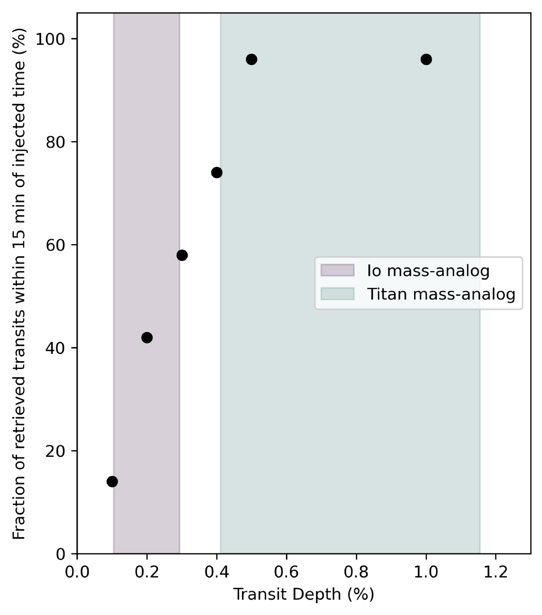
biosignatures in Earth's atmosphere

Figure 1: Atmospheric biosignatures present in Earth’s atmosphere. More abundant biosignatures include oxygen and ozone (byproducts of photosynthesis in plants and bacteria) and nitrous oxide (byproduct of bacteria that don’t need oxygen to survive). Less abundant biosignatures include isoprene (released from the breakdown of leaves that have fallen from trees) and sulfur gases (byproducts of cyanobacteria). [Kaz Gary]

There are many ways to observe the spectrum of a planet, but the one you’re probably most familiar with is transmission spectroscopy. You can learn more about transmission spectroscopy of exoplanet atmospheres and how to model transmission spectra with these bites: 1, 2, 3. However, all of the current techniques for exoplanet spectroscopy (including transmission spectroscopy) measure the star’s light and how the planet affects the star’s light. This means it’s heavily dependent on how we model the star’s light to indirectly observe the planet’s light. The only way to take the spectrum of a planet directly is with direct imaging: the technique that the future Habitable Worlds Observatory will use to find signs of life in planetary spectra.

But are atmospheric biosignatures the only way to tell if life exists on other planets? Short answer: absolutely not. Let’s take Earth as an example. If we imagine Earth as a directly imaged exoplanet and take spectra of the light it reflects, you’ll find that around near-infrared wavelengths (~700 nanometers or just past the red part of the visible light spectrum), the light reflected off of Earth increases sharply. This sharp increase is called the vegetation red edge and is caused by plant and ocean life on Earth’s surface as shown in Figure 2. This is made possible because chlorophyll (the thing that makes plants green) absorbs nearly all visible light but reflects near-infrared light. The vegetation red edge is an example of a surface biosignature. In today’s article, the authors determine if the vegetation red edge will be visible in spectra of Earth-like exoplanets!

Spectra of different sources of the vegetation red edge

Figure 2: Spectra of different sources of the vegetation red edge on Earth. The vegetation red edge is highlighted in gray where the spectra rapidly increase and then level off beyond the visible light part of the spectrum. Each color represents a different source with pictures of each source on the right-hand side of the plot. [O’Malley-James and Kaltenegger 2019]

Snapshots

Planets rotate; that’s how we have morning, noon, and night in 24 hours guaranteed. This means that different parts of the surface will be visible at different times when we take spectra. Sometimes, we may see more ocean than land, other times not. To determine if the vegetation red edge would be visible at all points in Earth’s day, the authors simulated nine different spectra of modern-day Earth representing nine snapshots of Earth’s rotation. Additionally, they also simulated a time-averaged spectrum that shows an entire Earth day in one snapshot without the time variability. These spectra are shown in Figure 3.

Spectra of a directly imaged modern-day Earth at nine different times in its rotation

Figure 3: Spectra of a directly imaged modern-day Earth at nine different times in its rotation. The y-axis is the ratio of the planet’s signal to the star’s signal and the x-axis is wavelength in microns. Each color represents a time in UTC and the black curve represents the time-averaged spectrum. [Burr et al. 2026]

The authors then run retrieval models on all nine spectra to see if the vegetation red edge would be detectable in each spectrum, including the time-averaged one. Retrieval models take into account characteristics of the planet that would affect how light moves through its atmosphere, such as the atmospheric chemicals present and the surface gravity. They then use this information to generate possible spectral models that could fit the data. The best-fit model allows astronomers to infer what the atmosphere is made of and properties of the planet such as surface gravity. Because we are looking at Earth in visible light, much of the light from the planet is reflected. Typically, models of Earth-like planets in visible wavelengths only include atmospheric albedo: the measure of how reflective a planet’s atmosphere is. However, surface biosignatures can also be reflective as shown by the vegetation red edge. The authors use this to their advantage and introduce a surface albedo into their model that changes with the amount of desert, vegetation, and ocean visible on Earth’s surface at that time. They then further divide the nine spectra into three different types based upon the visible surface: majority land; 50% land, 50% ocean; and majority ocean. Check out the article online to see a cool animation of the Earth rotating and how the spectrum looks different at each time!

Arr! There Be… Vegetables?

After running the models, the authors were able to detect a sharp increase in the surface albedo value in every spectrum, including the time-averaged one. This result is shown in Figure 4. The authors take this result one step further in order to validate that the vegetation red edge is actually a result of surface variation of vegetation. They re-run models on each of their spectra but instead include a constant surface albedo instead of a time-varying one. This resulted in incorrectly measured radii, chemicals, and surface gravity in nearly all of the models. Without the vegetation red edge and surface features, the models could not accurately determine if life was present on Earth.

Retrieved surface albedos for the nine time-varying spectra

Figure 4: Retrieved surface albedos for the nine time-varying spectra. The surface albedo is broken down into three different values (a₁, a₂, a₃). Each of these values represents a change in the surface albedo at different wavelengths (i.e., how reflective the surface is at three different wavelengths). The nine spectra were broken down by the amount of surface that was visible at that time and color-coded for each category. The time-averaged spectrum is shown in gray. Each category of spectra was able to retrieve an increase in reflected light from the surface at vegetation red edge wavelengths. The spectra that had the majority land visible have the biggest increase in the surface albedo. This makes sense since the amount of visible vegetation is the largest with majority-land planets. [Burr et al. 2026]

For the first time (to the author’s knowledge), the vegetation red edge has been shown to be a promising and observable biosignature in Earth-like atmospheres. This study has also laid the groundwork for future work on other surface biosignatures and their potential impact on spectra of habitable planets. Confirming signs of life in multiple different ways, both on the surface and in the atmosphere, will finally allow astronomers to say we are not alone in the universe. In fact, life likes to live on the (red) edge!

Original astrobite edited by Madison VanWyngarden.

About the author, Kaz Gary:

I am a fourth-year PhD candidate at The Ohio State University with a passion for planets. My current work focuses on modeling exoplanet observations for the Habitable Worlds Observatory and understanding planetary atmospheres. Outside of research, I help develop planetarium shows and love all forms of science communication. In my free time, I enjoy playing tabletop RPGs, painting, watching terrible reality TV, and hanging out with my pet hedgehog.

The post Life on the (Red) Edge appeared first on AAS Nova.

  •  

I Spy with My Large Binocular Eyes: A Dusty Torus Around a Supermassive Black Hole?

NGC 4151

Editor’s Note: Astrobites is a graduate-student-run organization that digests astrophysical literature for undergraduate students. As part of the partnership between the AAS and astrobites, we occasionally repost astrobites content here at AAS Nova. We hope you enjoy this post from astrobites; the original can be viewed at astrobites.org.

Title: Shocks, Winds, and a Torus: The Large Binocular Telescope Interferometer (LBTI) Resolves the Active Nucleus of NGC 4151
Authors: Jacob W. Isbell et al.
First Author’s Institution: University of Arizona
Status: Published in ApJ

At the centre of nearly every galaxy lies a supermassive black hole that dominates this innermost region. Not only is there this millions-of-solar-masses dark beast, but usually too a whole bunch of stuff — stars, gas, dust, and more — which is often quite bright! When there is plenty of this material quite close to the black hole, we believe physics takes control to flatten it into a family of disk and toroidal structures in what we call the unified model of active galactic nuclei (AGNs; see Figure 1).

schematic of the unified model of active galactic nuclei

Figure 1: The unified model of AGNs asserts that there is an inner accretion disk, surrounded by a dusty torus that cohabitates with clouds moving at different velocities (the so-called broad and narrow line regions), and sometimes even relativistic jets extending from the accretion disk to galactic scales; you can read more about AGN structure in this Astrobites guide. [Emma Alexander; CC BY 4.0]

When astronomers look at different active galaxies (read: galaxies with active supermassive black holes at their core), we see a range of phenomenologies related to their brightness, spectra, morphologies, and more. The unified model of AGNs seeks to explain these different AGN appearances simultaneously by positing that they all have the same physical structure, and we are just viewing them from different angles, hence seeing different features.

The cores of AGNs are often imaged at the smallest scales (e.g., their accretion disks, viewed with interferometers like the Very Large Telescope Interferometer) and the largest scales (e.g., their relativistic jets, viewed with radio interferometers), but comparatively less effort has gone to directly observing the predicted dusty tori in the mid-infrared. That is exactly what today’s authors set out to do using the Large Binocular Telescope Interferometer (LBTI) — a pair of 8.4-metre-aperture mirrors separated by just over 14 metres and combined to simulate a telescope effectively 29 metres wide. This lets astronomers take direct images at a much higher resolution than a smaller-aperture telescope, and hence directly peer into the region around AGNs where this dusty torus should lie.

Today’s authors turn the LBTI towards NGC 4151, a medium-luminosity AGN. With the large effective aperture of the LBTI, they were able to resolve scales in the AGN region as small as 4.4–9.1 pc, about 14–30 light-years depending on the wavelength (see Figure 2), in the mid-infrared. These observations revealed warm dust emission in a complex structure around the central supermassive black hole. The authors note a central bar at all wavelengths, with a significant extension of cool dust arcing to the west (right in the image) and warmer dust localised to the centre (as evident by 3.7- and 4.8-micron emission only nearest to the supermassive black hole and its accretion disk).

deconvolved images of the AGN core of NGC 4151

Figure 2: The deconvolved images of the AGN core of NGC 4151 show a very bright central source (the innermost region around the supermassive black hole), as well as some complex surrounding structure particularly at long wavelengths. The interpreted morphology is described in Figure 3. These images are deconvolved, meaning that known optical effects are corrected for on the raw data to produce a sharper image. [Adapted from Isbell et al. 2026]

To explain the observed morphology in Figure 1, the authors compare three different interpretations based on this new high-resolution imagery together with the results of previous studies looking at other scales and the spectrum of the AGN core. Each interpretation is illustrated and briefed in Figure 3.
illustration of the different regions surrounding NGC 4151's black hole and potential interpretations for the observed morphology

Figure 3: Three interpretations of the observed morphology are presented by the authors. The left panel illustrates the different regions surrounding the supermassive black hole (together with the results of other studies cited in the article). The right panel shows the suggested interpretations explaining the morphology. [Isbell et al. 2026]

The first interpretation is in keeping with the unified model of AGNs: a geometrically and optically thick torus of dust surrounds the inner region. In this interpretation, the surface of the dusty torus re-radiates light from the accretion disk to produce most of the mid-infrared emission. Additional mid-infrared emission could come from localised concentrations of gas or interactions between the outflow and the jet. The authors immediately disfavour this explanation, as other studies have shown bright ionised emission at the location of the would-be torus, which is not expected if an optically thick torus were to be present. Hence, these new observations somewhat challenge the one “flavour” of the unified model of AGNs.

The second interpretation aligns with a different version of the unified model: one in which a geometrically thin disk replaces a thick torus around the AGN core. Provided the disk is optically thin too, the authors favour this approach as it is consistent with the geometry of ionised emission that worked against the first interpretation. While other studies suggest that this thin disk should be optically thick, this morphology is at least better aligned with what we see in other AGNs.

The third interpretation suggests that the emission comes from only the radiation pressure–driven wind emanating from the AGN core. The authors disfavour this explanation, citing previous radiative transfer simulations that show that the flux should fall off with distance from the core too quickly to be consistent with the observations.

No matter the interpretation, these LBTI observations are an important glimpse into the future of mid-infrared AGN studies that will be done with 30-metre-class telescopes (such as the European Southern Observatory’s Extremely Large Telescope). This article, together with the group’s similar study on NGC 1068, is challenging and refining an accepted view of AGN morphology — the consequences of which apply to galaxies near and far — and poses new questions perfect for sophisticated hydrodynamic and radiative simulations.

Original astrobite edited by Margaret Verrico.

About the author, Ryan White:

I am a first-year PhD student at Macquarie University in Australia, working mainly on binary/multiple systems with massive stars (Wolf–Rayets in particular!). Outside of study, I’m probably drinking coffee, baking, reading, or going for a run. You can also find me procrastinating on Bluesky @astroryan.bsky.social.

The post I Spy with My Large Binocular Eyes: A Dusty Torus Around a Supermassive Black Hole? appeared first on AAS Nova.

  •  

Hunting for Exomoons Around a Lonely Planet

illustration of an exoplanet and exomoon around a star

Editor’s Note: Astrobites is a graduate-student-run organization that digests astrophysical literature for undergraduate students. As part of the partnership between the AAS and astrobites, we occasionally repost astrobites content here at AAS Nova. We hope you enjoy this post from astrobites; the original can be viewed at astrobites.org.

Title: A Deep Search for Exomoons Around WISE 0855 with JWST
Authors: Mikayla J. Wilson et al.
First Author’s Institution: University of California, Santa Cruz
Status: Published in AJ

The “Moon”-umental Question

The solar system hosts hundreds of moons, ranging from volcanic worlds like Io around Jupiter, to icy objects like Enceladus around Saturn, to captured objects like Neptune’s retrograde moon Triton. Moons are essential to our model of how the solar system formed and also offer some of the best chances we have for finding life beyond Earth.

Astronomers also expect exomoons, or moons orbiting planets outside the solar system, to be abundant around other giant exoplanets. But how common are exomoons? How do they compare to the moons in our solar system?

In order to begin answering those questions, we must first detect an exomoon, which has proved difficult despite decades of searching by astronomers. Fortunately, JWST presents a new opportunity to uncover the exomoon population by looking at lonely free-floating planets as they drift through space.

Why Free-Floating Planets?

One proposed method for searching for exomoons is by looking for their transits in front of their host planets, characterized by the dips in brightness of the planet as the moon passes in front, blocking the planet’s light. Looking for exomoon transits around planets orbiting stars is quite difficult, as the bright starlight can easily drown out the small signals of exomoon transits. Free-floating planets solve this issue by removing the star entirely, increasing our sensitivity to such detections. (See this bite for a good review.)

The authors of today’s article directed the exomoon hunt towards the free-floating WISE J085510.83-071442.5 (or WISE 0855). It has the prestige of being the coldest known brown dwarf (250–285K) while also sitting at a relatively low mass (3–10 Jupiter masses). Notably, it is also one of our closest neighbors at a distance of only 7.4 light-years, making it ideal for high-precision observations despite its faintness. Even though brown dwarfs are technically distinct from planets, the authors opt to refer to companions around WISE 0855 as moons given WISE 0855’s “planetary-mass” status. (It’s complicated…)

Repurposing JWST Data… for Moons!

The JWST observations used in this study contain 11 hours of near-infrared (2.87–5.27 microns) time-series spectra originally intended to study water clouds and weather on WISE 0855. Time-series brightness monitoring can also be used for transit searches, which the authors take advantage of.

One complication is that WISE 0855 is variable, meaning its intrinsic brightness changes over time. Variability is likely driven by clouds and other dynamic processes within its atmosphere. So how do the authors distinguish between a passing moon and a turbulent atmosphere? The key idea is that variability is wavelength dependent, meaning that the brightness of WISE 0855 will fluctuate differently depending on the observed wavelength. In contrast, transits are “gray,” meaning that the same amount of light is blocked at all wavelengths, producing a consistent feature across the entire spectrum.

Finding Moons with Statistics!

The authors apply this idea and pick out two wavelength regions of WISE 0855’s spectrum that contain two distinct variability patterns, which should both contain an identical moon transit signal (if present). They then generate a light curve (how brightness changes over time) for these two regions (see Fig. 1).

WISE 0855 light curves

Figure 1: (A) Light curves from two selected wavelength regions of WISE 0855’s spectrum with injected transit signals. Also plotted is the best-fit Gaussian processes + transit model for the two light curves. (B) Light curve data after subtracting the Gaussian processes portion of the best-fit model, revealing the example injected transit signals. [Wilson et al. 2025]

To appropriately model the variability, the authors employ Gaussian processes, a flexible tool that can model complex, quasi-periodic signals like atmospheric variability. They compare fits from two types of models:
  • Gaussian processes–only model: Assumes that all observed variability is intrinsic to the planet itself
  • Gaussian processes + transit model: Includes a simple trapezoidal exomoon transit signal that is simultaneously fit in both light curves

Using Bayesian evidence (a measure of how well each model explains the data), they determined which model was favored. So, what do they find?

The Bad News and the Good News

Based on Bayesian evidence, the authors conclude that there are no statistically significant detections of exomoons in the data. The results suggest very weak evidence for a ~0.53-Earth-radius moon at a wide separation from WISE 0855 — an unlikely scenario given that transit probability decreases at greater separations (and therefore longer orbital periods).

Yet, the study goes further: What kinds of moons is JWST able to detect, if any? To answer this, the authors performed injection and recovery tests, where they injected artificial transit signals of varying depths (exomoon sizes) into the data and tested how well their models were able to recover them (results shown in Fig. 2). They find that JWST is capable of detecting 96% of transits with depths ≥0.5%, equivalent to a Titan-like moon. Smaller Io-like moons were also detectable more than half of the time. This means that if a Titan analog had actually transited during these observations, we would almost certainly have seen it!

plot of successful detections of injected transit signals

Figure 2: Results showing the number of successful detections for the transit injection and recovery tests. Fifty transit injections are done for transit depths of 1%, 0.5%, 0.4%, 0.3%, 0.2%, and 0.1%. The transit depths represent different exomoon sizes, with the shaded regions representing Io-like and Titan-like moons. [Wilson et al. 2025]

JWST will continue to gather more time-series data of free-floating planets, brown dwarfs, and directly imaged exoplanets, each providing a new opportunity to help us better understand the moon population outside of our solar system. We’re still waiting for the first confirmed exomoon, but when that transit finally happens, we know that JWST will be ready.

Original astrobite edited by Kelsie Taylor.

About the author, Jared Bull:

I am a 2nd-year PhD student at Johns Hopkins University. I study brown dwarf variability and am interested in using time-series observations to uncover dynamic processes within their atmospheres. In my free time I like to read, cook, and do astrophotography.

The post Hunting for Exomoons Around a Lonely Planet appeared first on AAS Nova.

  •  

Feed the Fire, Fade the Metals

galaxy cluster MACS J1149.5+2223

Editor’s Note: Astrobites is a graduate-student-run organization that digests astrophysical literature for undergraduate students. As part of the partnership between the AAS and astrobites, we occasionally repost astrobites content here at AAS Nova. We hope you enjoy this post from astrobites; the original can be viewed at astrobites.org.

Title: Metal-Poor Star-Forming Clumps in Cosmic Noon Galaxies: Evidence for Gas Inflow and Chemical Dilution Using JWST NIRISS
Authors: Vicente Estrada-Carpenter et al.
First Author’s Institution: Arizona State University
Status: Published in ApJ

If you want to reconstruct a galaxy’s life story, one of the best “fossil records” is its metallicity. In astronomy this refers to the abundance of elements heavier than helium, which are made in stars and returned to a galaxy’s gas through winds and supernovae. Over time, more star formation usually means more metals mixed into the gas.

Now zoom to Cosmic Noon (roughly when the universe was most actively forming stars). Many galaxies in this epoch look “clumpy”; their star formation is concentrated in several bright knots scattered across the disk. The big question is where those clumps come from. Do they form from the galaxy’s own gas via internal disk instabilities, or do they light up when fresh, metal-poor gas flows in and both fuels star formation and dilutes the local metallicity?

The authors try to answer that question with JWST by measuring the metallicity of each clump relative to its immediate surroundings, rather than comparing clumps to a single galaxy-wide number (which can be misleading if the galaxy has a metallicity gradient).

They use JWST/Near Infrared Imager and Slitless Spectrograph (NIRISS) slitless grism spectroscopy from the CAnadian NIRISS Unbiased Cluster Survey (CANUCS) to study 20 lensed galaxies at redshift 0.6 < z < 1.35. (Lensing effectively acts like a zoom lens, helping to resolve smaller structures.) They focus on emission lines that trace star-forming gas, especially Hα (a star formation tracer) and sulfur lines [SII] and [SIII] (needed for their metallicity method).

Slitless spectra come with a headache: because there is no slit, different parts of a galaxy can overlap in the dispersed image. To make reliable emission-line maps from slitless data, the authors use a forward-modeling code called Sleuth, which allows the continuum to vary across the galaxy.

The authors identify clumps using the Hα map together with rest-frame ultraviolet imaging because these tracers are sensitive to star formation on different timescales: Hα highlights gas ionized by the youngest massive stars, while ultraviolet light traces young stellar light over longer periods. As a result a clump can be bright in one and not the other, especially if dust is involved.

To estimate gas-phase metallicity, they use the “strong-line” method, which infers metallicity from ratios of bright emission lines calibrated using models and empirical samples. Their main diagnostic is S23 = ([SIII] + [SII]) / Hα. Because some line ratios also depend on the ionization state (how strongly the gas is being ionized by young stars), they also use the sulfur ratio S32 = [SIII]/[SII] as a check and iterate to a self-consistent solution.

So, Are Clumps Really Chemically Different from Their Surroundings?

For each clump, the authors measure the metallicity inside the clump and compare it to an annulus just outside the clump (masking neighboring clumps to avoid mixing). When they plot “clump metallicity” versus “local disk metallicity,” most points fall below the 1-to-1 line, meaning the clumps are more metal poor than their surroundings (Figure 1). The mean offset is about 0.1 dex, which corresponds to roughly 20% dilution in the clump gas.

plot of gas-phase metallicity in star-forming clumps compared against metallicity of nearby disk regions

Figure 1: Each point compares a star-forming clump’s gas-phase metallicity to the metallicity of the nearby disk region immediately surrounding it. If clumps and disks had the same metallicity, they would lie on the dashed 1-to-1 line. Instead, most clumps sit below it, showing a typical ∼0.1 dex metallicity deficit, consistent with local chemical dilution. (The solid red line shows a best-fit linear trend to the clump measurement.) [Adapted from Estrada-Carpenter et al. 2025]

An extra wrinkle is that the galaxy medians hint at two populations: some galaxies have clumps with small offsets (near the 1-to-1 line), while others show larger offsets. The authors suggest this could mean two formation pathways, one dominated by internal gas reservoirs (smaller offsets) and another where inflow of metal-poor gas plays a bigger role (larger offsets). They are careful, though, as the sample is still small.

If inflow is really the driver, you should expect a link: the more strongly a clump is forming stars relative to its surroundings, the more diluted its metallicity should be. That is exactly what the authors find. The clumps that are most boosted in star formation are also the most metal diluted.

The article also emphasizes that clumps are not chemically uniform blobs. In at least one detailed example, the peaks in Hα (highest star formation) coincide with local minima in metallicity along a cut through the galaxy (Figure 2), suggesting internal star formation rate and metallicity gradients that reinforce the same story, intense star formation goes hand in hand with lower metallicity in the clump regions.

galaxy image showing spatial variation of H alpha and metallicity

Figure 2: Example galaxy from this study illustrating the clump-scale link between star formation and metallicity. The color image shows the galaxy with a rectangular strip marking the region used for a 1D cut. In the bottom panel, the turquoise line shows the Hα flux (a tracer of recent star formation), while the white line shows the metallicity along the same cut. Peaks in Hα flux line up with local dips in metallicity, showing that the brightest star-forming clumps are also the most chemically diluted compared to nearby regions. [Adapted from Estrada-Carpenter et al. 2025]

Are These Clumps Really “In Situ,” or Could They Be Small Satellites?

A reasonable alternative is that some clumps are actually small companion galaxies projected onto the disk. These could also look metal poor, because low-mass galaxies tend to be low metallicity. The authors look for evidence using face-on systems and find that more massive clumps tend to sit closer to galaxy centers, which is consistent with in-situ clumps that form in the disk and migrate inward, though it does not rule out satellites. They argue that kinematics from JWST/NIRSpec IFU will be needed for a definitive separation.

Why This Matters

Gas inflow, star formation, and feedback, together known as the baryon cycle, are key drivers of how galaxies grow. What this article adds is a spatially resolved view that compares each clump to its local environment, showing that regions of elevated star formation also tend to be locally metal poor. That pairing is hard to explain as a simple metallicity gradient or a galaxy-wide averaging effect, and it is exactly what you would expect if at least some clumps are being fueled by relatively metal-poor inflows. In short, these clumps may be snapshots of galaxies refueling in real time.

Original astrobite edited by Ryan White.

About the author, Niloofar Sharei:

I’m an astronomy PhD candidate at UC Riverside studying how galaxies grow through star-forming clumps. I track how these clumps emerge, evolve, and sometimes survive long enough to reshape their galaxies. When I’m not thinking about cosmic blobs, I’m reading, hiking, or listening to Bach.

The post Feed the Fire, Fade the Metals appeared first on AAS Nova.

  •  

The Oldest Starlight

illustration of stars in the early universe

Editor’s Note: Astrobites is a graduate-student-run organization that digests astrophysical literature for undergraduate students. As part of the partnership between the AAS and astrobites, we occasionally repost astrobites content here at AAS Nova. We hope you enjoy this post from astrobites; the original can be viewed at astrobites.org.

Title: Hunting for the First Explosions at the High-Redshift Frontier
Authors: Junehyoung Jeon et al.
First Author’s Institution: The University of Texas at Austin
Status: Published in ApJ

Back in the 1920s, astronomers discovered that we live within just one of many, many galaxies in the big, wide universe. Since then, we’ve been racing to search for the most distant galaxy that can be observed — in other words, searching for the oldest starlight we can see, since the light from these distant sources has been travelling towards us for most of the age of the universe. (Remember: more distant = higher redshift = longer lookback time.)

This race to the redshift frontier has had a pretty eventful history (see a great overview video here), which became even more eventful with the launch of JWST. JWST rapidly smashed the previous redshift (z) record of z = 10.6 by discovering a galaxy at z = 13.2, and then it broke its own record twice more. The current title holder sits at z = 14.4, observed less than 300 million years after the Big Bang.

Several galaxy candidates (to date unconfirmed) have now even been proposed at z ~ 25–32 (e.g., Capotauro), only 100 million years after the Big Bang! If real, these sources would pose a serious challenge to our understanding of the formation of the first galaxies, as galaxies shouldn’t really be observable at such early times. In today’s article, the authors put forward an intriguing alternative: what if some of these ultra-high-redshift candidates aren’t galaxies at all, but transient explosions from the universe’s first stars?

The First Stars and Their Explosive Endings

The earliest generation of stars (Population III; see my previous bite on these here) formed from pristine hydrogen and helium gas. Without metals to cool the gas efficiently, theory predicts that these stars were extremely massive, often exceeding 100 solar masses. While such stars would be short-lived, their deaths could be spectacular.

Population III stars of sufficient mass are predicted to end their lives as hyper-energetic pair-instability supernovae (PISNe). This is a long-winded name for a rapid, intensely hot explosion that leaves no remnant behind — not even a trace of the pre-existing star. Whilst nothing would remain of the star, the light emitted in that explosion could be bright enough to masquerade as a high-redshift galaxy candidate in current JWST surveys, but only if three key conditions are met:

  1. JWST must observe a sufficiently overdense region, where lots of Population III stars can form very early.
  2. A PISN must occur while JWST is “watching.”
  3. The explosion must be bright enough to rise above JWST’s detection limits.

Simulating a (Biased) Universe

To address the likelihood of these conditions having already been met by existing JWST observations, the authors turn to cosmological simulations. Rather than simulating an “average” patch of the universe, they focus on an extremely overdense region (Fig. 1). This creates a rare but important environment where structures collapse earlier than usual. These regions are exactly where large numbers of Population III stars are expected to form at the highest redshifts.

projection of the gas density in the simulated overdense region at z = 30.4

Figure 1: A projection of the gas density in the simulated overdense region at z = 30.4. The densest structures stand out clearly, tracing the locations where the first stars are able to form. Black dots mark newly formed groups of stars, while the most massive dark matter halo in the region is highlighted with an orange circle. The figure illustrates that in such an unusually dense patch of the early universe, star formation can already be underway just 100 million years after the Big Bang, creating the conditions needed for early Population III stars and their explosive deaths. [Adapted from Jeon et al. 2026]

In their simulations, star formation begins as early as z ~ 30–40 (within the first hundred million years after the Big Bang), producing Population III stars and, by extension, potential PISNe very shortly afterwards. While such overdense regions are rare, the authors show that the total area already surveyed by JWST (including large surveys such as CEERS, JADES, PRIMER, and COSMOS-Web) is large enough that it is plausible JWST has already observed at least one such region.

Catching a Cosmic Explosion in the Act

So, we can tick off condition #1: it’s possible that a sufficiently overdense region has already been observed by JWST. Next up, how lucky do we have to be to catch an explosion in the act (condition #2), so to speak? For this condition, cosmic time dilation actually works in our favour. A PISN explosion at z > 20 that lasts only months in its own rest frame can last for decades in the observed frame. (This whole time-being-relative thing sounds wacky because it is — please join me, Neil deGrasse Tyson, and countless others in struggling to imagine this.)

But would any such explosion be bright enough (condition #3)? Using theoretical PISN spectra, the authors show that these explosions could reach observed magnitudes of ~28–29 at z ~ 30 — right at the depth of current JWST deep surveys (Fig. 2). In fact, the predicted brightness and colours are somewhat comparable to those of some proposed z ~ 30 candidates (Fig. 3), raising the possibility that these objects could be PISNe rather than galaxies.

plot of predicted PISN brightness

Figure 2: This plot compares the predicted brightness of PISNe originating from different types of extremely massive stars to the depth reached by existing JWST surveys, showing that these explosions could remain detectable for ~20 years at peak brightness in the observed frame. [Jeon et al. 2026]

Theoretical PISNe spectra compared to a proposed z = 32 source

Figure 3: A comparison of theoretical PISNe spectra with the observed photometry of one proposed z ≈ 32 source (Capotauro). The coloured curves show model spectra for PISNe originating from extremely massive stars, at different stages of the explosion, while the data points represent the observed brightness of the high-redshift candidate across multiple JWST filters. [Jeon et al. 2026]

So… Are We Seeing the First Stars Die?

It’s not time to throw a party just yet. The authors note there are several caveats and uncertainties. The nature of Population III stars is still highly uncertain, JWST does not continuously monitor the same patch of sky, and identifying a PISN at such high redshift would be extremely challenging. Thanks to time dilation, these explosions would fade very slowly, making them hard to distinguish from steady sources using photometry alone. Alternatively, there are other plausible explanations for these ultra-high-redshift candidates: lower-redshift interlopers (a rather infamous example is CEERS-93316), local brown dwarfs, or even nearby exoplanets.

Still, the idea is exciting. If JWST were to detect a genuine PISN at z > 20, it would represent a direct glimpse of the very first stars, pushing observational astronomy into truly uncharted territory. For now, the most distant explosions in the universe may already be hiding in JWST images; we just have to learn how to recognise them.

Original astrobite edited by Nathalie Korhonen Cuestas.

About the author, Lucie Rowland:

I’m a fourth (and final!) year PhD student at Leiden Observatory in the Netherlands, studying massive, star forming galaxies in the early universe with ALMA and JWST. It’s a really exciting time to be interested in astronomy, so I hope to make groundbreaking new research more accessible!

The post The Oldest Starlight appeared first on AAS Nova.

  •  

A Possible GLIMPSE of the Universe’s First Stars

Population III stars

Editor’s Note: Astrobites is a graduate-student-run organization that digests astrophysical literature for undergraduate students. As part of the partnership between the AAS and astrobites, we occasionally repost astrobites content here at AAS Nova. We hope you enjoy this post from astrobites; the original can be viewed at astrobites.org.

Title: GLIMPSE: An Ultrafaint ≃105 M⊙ Pop III Galaxy Candidate and First Constraints on the Pop III UV Luminosity Function at z ≃ 6–7
Authors: Seiji Fujimoto et al.
First Author’s Institution: University of Toronto; The University of Texas at Austin
Status: Published in ApJ

You, me, your laptop, my $8 matcha, and just about everything else on Earth was forged in the fiery bellies of dying stars. Generations of stars had to live and die before the universe became enriched with any elements heavier than helium (what astronomers call “metals”). The first stars to undergo this cosmic cycle are known as Population III (Pop III) stars. Though their existence has been hypothesized since the 1960s, astronomers have failed to observe these distant metal-free stars or the faint, low-mass galaxies that host them.

The first Pop III stars likely formed around 100 million years after the Big Bang in pristine pockets of hydrogen gas. Although these are too distant for us to observe, we expect that as the universe started to become metal enriched, there were still existing pockets of gas introverted enough to survive unpolluted and form metal-free Pop III stars up to a redshift of z ~ 6–7 (when the universe was around 900 million years old)!

JWST is the perfect instrument to search for these systems. You can read other astrobites on the search for possible Pop III systems with JWST here and here. The authors of today’s article seek to develop the most efficient way of using JWST’s Near-Infrared Camera (NIRCam) to find the galaxies hosting Pop III stars. Using their selection method on existing NIRCam data, the authors identified one promising Pop III galaxy candidate.

I’m Not Like Other Galaxies

In order to find a Pop III galaxy, we need to take a look at galaxies’ spectral energy distributions (SEDs). These are graphs that show the energy emitted by a galaxy at different wavelengths of light. Pop III galaxies are expected to have SEDs that differ from your everyday, metal-enriched galaxy. NIRCam will be especially sensitive to three key spectral features that show up in the SEDs of Pop III galaxies: an absent [O III] line (light emitted by doubly ionized oxygen atoms), a strong H-alpha line (light emitted when a hydrogen atom transitions from its third to its second energy level), and a significant Balmer jump (light absorbed to ionize electrons in the second energy level of a hydrogen atom). To identify these key SED characteristics, the authors use SED fitting and color–color diagrams to execute an efficient Pop III search with NIRCam.

The first selection method involves SED fitting. Astronomers create template SEDs that represent different types of galaxies and then compare these templates to the observed SEDs to see which one matches best. In this work, the authors use metal-rich galaxy templates and Pop III templates to fit the galaxies observed with NIRCam. They then calculate the chi-squared χ2 (a statistical measure of best fit) between the data and all the SED templates. A galaxy is selected as a Pop III candidate if the Pop III model provides a good fit (χ2 < 10) to the photometry and is significantly better than any metal-rich model. It’s kind of like looking for Cinderella by making every woman in the kingdom try on the glass slipper.

A color-color diagram showing how Pop III models lie in a different parameter space than metal-rich galaxies.

Figure 1: Color–color diagram for selecting Pop III galaxies where the x and y-axes show the different NIRCam filters being subtracted. The cyan symbols are different Pop III models while the other colored dots are different metal-rich galaxy models. [Adapted from Fujimoto et al. 2025]

A color–color diagram plots the difference in magnitude between two filters on each axis. NIRCam filters are specially chosen to emphasize the SED characteristics above. When these filters are chosen, Pop III galaxies occupy a distinct region of this diagram as compared to metal-rich galaxies. For example, subtracting the F356W filter from the F277W filter is sensitive to the presence of the [O III] line and the Balmer jump. Figure 1 demonstrates how this color selection separates Pop III galaxies from typical galaxies.

O Pop III, Pop III, Wherefore Art Thou?

The authors apply their fresh new selection criteria to publicly available NIRCam data from large surveys. And (drum roll please) the slipper fits! The Pop III galaxy candidate GLIMPSE-16043 is an ultra-faint galaxy at z = 6.5. It was imaged in the GLIMPSE survey, which uses the technique of gravitational lensing to observe faint and distant galaxies.

The GLIMPSE survey targeted a massive galaxy cluster, Abell S1063. The cluster bends the light from distant galaxies and, like a giant lens, magnifies faraway objects, providing some of the deepest JWST imaging to date. The Pop III candidate passes both tests: it resides in the Pop III region of the color–color diagram, and its SED is best fit by a Pop III model, not a metal-rich galaxy model (see Figure 2). Next, spectroscopic follow-up is needed to ensure that this galaxy is truly metal free and not just extremely metal poor.

The spectral energy distribution of a Pop III galaxy candidate. This plot shows that the JWST data is best fit by a Pop III model rather than a metal-rich galaxy.

Figure 2: SED of GLIMPSE-16043 with the best-fit Pop III template (blue) and best-fit metal-enriched template (gray). The top panel is the galaxy imaged in different filters from NIRCam and the Hubble Space Telescope. [Fujimoto et al. 2025]

The authors conclude that our best shot at identifying additional Pop III galaxy candidates is using NIRCam to image large numbers of gravitationally lensed clusters. Without magnification from gravitational lensing, it may be impossible to see these ultra-faint Pop III galaxies. Once candidates have been identified, they can be followed up with deep spectroscopy to confirm their redshift and their lack of metals. Who knows? With these new methods, we may soon get a glimpse of the universe’s very first stars.

Original astrobite edited by Chris Layden and Margaret Verrico.

About the author, Madison VanWyngarden:

I am a first-year PhD student in astronomy and NSF Graduate Research Fellow at the University of Arizona. I study galaxy formation and evolution in the distant universe and am particularly interested in dusty star-forming galaxies. In my free time, I love reading, hiking, and baking bread!

The post A Possible GLIMPSE of the Universe’s First Stars appeared first on AAS Nova.

  •  

Observing the End of Star Formation in Galaxies

galaxy transitioning from star forming to quiescent

Editor’s Note: Astrobites is a graduate-student-run organization that digests astrophysical literature for undergraduate students. As part of the partnership between the AAS and astrobites, we occasionally repost astrobites content here at AAS Nova. We hope you enjoy this post from astrobites; the original can be viewed at astrobites.org.

Title: Searching Within Galaxies for the Earliest Signs of Quenching With Spatially Resolved Star Formation Histories in UVCANDELS
Authors: Charlotte Olsen et al.
First Author’s Institution: New York City College of Technology
Status: Published in ApJ

How and Why Do Galaxies Stop Forming Stars?

Galaxies serve as important laboratories for many subfields of astrophysics. As such, astrophysicists are interested in the full galactic life cycle, from how galaxies are born to the end of their formation. Whereas young galaxies in the distant universe are actively forming stars, many nearby galaxies are much quieter, with little or no ongoing star formation. Astronomers like to describe these galaxies as “red and dead” because their stars are older and therefore appear redder in color. The process by which galaxies shut down their star formation is known as quenching, and it causes galaxies to become quiescent. Understanding the origin of quiescent galaxies is a fundamental question in galaxy evolution. Studying this process is challenging, however, because star formation is intertwined with many other factors that shape galaxies, including their environments and supermassive black holes.

Star formation occurs on scales that are much smaller and over timescales much shorter than the global properties and overall lifetime of a galaxy. By observing star formation on these smaller scales over time, astronomers can gain a clearer picture of how star formation ceases in a galaxy, and they can determine whether this process is driven from the inside out — starting with the supermassive black hole in the galactic center — or from the outside in, influenced by environmental effects. In today’s article, the authors use the Cosmic Assembly Near-Infrared Deep Extragalactic Legacy Survey with high-resolution ultraviolet coverage (UVCANDELS) to examine eight “golden” galaxies, shown in Figure 1. They then reconstruct the star formation histories within small regions of each galaxy to detect the “earliest signs of quenching.”

galaxy sample from Olsen et al.

Figure 1: Images of the eight galaxies in the “Golden Sample” of galaxies studied in this work (right). These galaxies were chosen because of their clear detection, and they show a range of edge-on to face-on views as well as shapes. The authors divided each galaxy into small, resolved regions in which they measured the star formation (example shown on left). [Adapted from Olsen et al. 2026]

Characterizing the Star Formation Histories

To trace a galaxy’s star formation over cosmic time, today’s authors model its integrated light — which encodes the many episodes of past star formation — using spectral energy distribution (SED) fitting. By comparing a galaxy’s light across many wavelengths to computer models, SED fitting can estimate the ages of its stars and when they formed. This approach allows astronomers to study how a galaxy’s star formation rate evolves as a function of its stellar mass, known as the SFR – Mstellar relation. Note that the article considers the star formation rate and stellar mass in individual regions of each galaxy, so it analyzes these properties as surface densities, ΣSFR and ΣMstellar, instead of the total values.

Using SED fitting, the authors determine the expected star formation rate and stellar mass of the regions from 250 million to 1 billion years before the time of observation. Figure 2 shows the line of best fit for the SFR – Mstellar relation of the regions for each galaxy, before and at the time of observation. The SFR – Mstellar relations are very similar across the sample 1 billion years before the observations; however, by the time of observation, the overall star formation rates have decreased slightly, indicating that the galaxies are beginning to quench. They also exhibit increased variation suggesting that each galaxy is quenching in a different way.

best-fit SFR – M stellar relation

Figure 2: The best-fit SFR – Mstellar relation of the regions for each galaxy, represented by the different colored lines, 1 billion years (1 Gyr) before and at the time of observation (left and right panels, respectively). At 1 billion years before the observation, the galaxies appear to have the same relation, but their variation at the time of observation suggests that the galaxies have begun quenching in different ways. [Olsen et al. 2026]

To further probe how these galaxies are starting to quench, the authors also measure the specific star formation rate (sSFR) of the regions as a function of their distance from the center of the galaxy. The sSFR can be thought of as the rate of new star formation relative to the amount of existing stellar mass: SFR /Mstellar. Figure 3 shows three examples from the galaxies studied in this work. Once again, the star formation rates of the regions decrease over the course of 1 billion years. However, the regions where the star formation rate has declined most rapidly differ from galaxy to galaxy — ranging from the central regions to the mid-disk to the outskirts — as each galaxy is undergoing a different quenching mechanism.
specific star formation rate of the regions as a function of their distance from the center of the galaxy

Figure 3: The specific star formation rate of the regions as a function of their distance from the center for three of the galaxies in the sample. Overall, the star formation rate decreases from 1 billion years before the observation (red) to the time of observation (blue). However, the regions where the star formation decreases most significantly (indicated with the yellow boxes) vary from galaxy to galaxy. [Olsen et al. 2026]

Detecting the Earliest Signs of Quenching

It should be noted that all of the galaxies in this study are still forming stars. However, they are on the verge of having their star formation suppressed, offering valuable insight into how quenching begins and how diverse the process can be. New telescopes are pushing the boundaries of what we can observe. On one hand, JWST can capture galaxies at exceptionally high resolution; on the other, the Vera C. Rubin Observatory and the Nancy Grace Roman Space Telescope will deliver vast datasets containing billions of galaxies. Future investigations leveraging these facilities could reveal more about the physical processes that quench galaxies on small scales, shedding light on the mechanisms that drive galaxy evolution.

Original astrobite edited by Catherine Slaughter.

About the author, Shalini Kurinchi-Vendhan:

After studying astrophysics and literature at Caltech, I moved onto a Fulbright Fellowship in Heidelberg, Germany. I’m passionate about using computer simulations to explore supermassive black holes and galaxy evolution — but I also love poetry and traveling.

The post Observing the End of Star Formation in Galaxies appeared first on AAS Nova.

  •  

A Potential New Piece of the “Little Red Dot” Puzzle

X-ray dot

Editor’s Note: Astrobites is a graduate-student-run organization that digests astrophysical literature for undergraduate students. As part of the partnership between the AAS and astrobites, we occasionally repost astrobites content here at AAS Nova. We hope you enjoy this post from astrobites; the original can be viewed at astrobites.org.

Title: The X-Ray Dot: Exotic Dust or a Late-Stage Little Red Dot?
Authors: Raphael E. Hviding et al.
First Author’s Institution: Max Planck Institute for Astronomy
Status: Published in ApJL

What Are Little Red Dots?

One of the most intriguing results produced by JWST was the serendipitous discovery of a new class of object: “little red dots” (LRDs). These objects started popping up everywhere in our early universe observations. Surprisingly, they look like compact (little) red dots in imaging data (astronomers are an incredibly creative bunch). The number of LRDs we observe drops drastically at redshifts less than about z = 4 (about 12 billion years ago), implying that LRDs are likely evolving into something else entirely. The luminous, compact nature of LRDs, paired with their disappearance from the cosmic stage, has continuously puzzled astronomers in recent years.

At least part of the LRD population has routinely been explained as a new class of active galactic nuclei (AGN). AGN are the central engines of many galaxies — luminous regions powered by actively accreting supermassive black holes. Recent evidence has increasingly pointed towards LRDs being a new class of AGN: black hole stars, or black holes surrounded by dense cocoons of gas. Naturally, this raises questions surrounding the placement of LRDs in our understanding of supermassive black hole and galaxy evolution across cosmic time.

A hallmark of typical AGNs is their X-ray brightness. X-rays are one of the most energetic types of electromagnetic radiation, and they are primarily produced by the most extreme astrophysical situations (think neutron star mergers). One of the key challenges in explaining the nature of LRDs has been their lack of X-ray emission. Their lack of emission in this regime is a piece of evidence pointing towards a black hole star scenario — dense gas can block the X-rays being produced by the black hole. However, the lack of LRDs in the present-day universe implies that they likely shed their cocoons at some point. Catching an LRD in the act of shedding its cocoon would thus provide an important piece of evidence surrounding their nature and evolution. Thankfully, today’s authors may have done exactly that! They report the discovery of what they call the “X-ray dot” (XRD): an LRD-like object that is also X-ray luminous at a redshift of approximately z = 3.28.

New JWST Observations of the XRD

While archival observations of the XRD with the Hubble Space Telescope, the Canada France Hawaii Telescope, the Spitzer Space Telescope, and the Chandra X-ray Observatory existed, new spectral data from JWST were needed to study the system in depth. Spectral data have a huge advantage over photometric observations when it comes to modeling the system. With a good quality spectrum, astronomers can use sophisticated modeling tools to try and pin down the physical nature of the emission we’re observing, and thus understand its intrinsic nature.

Figure 1 showcases the archival data from Hubble, Spitzer, and Chandra, along with the XRD’s spectrum from JWST (black curve, bottom panel). Photometric observations of the source indicate that it is incredibly compact (radius ≲ 250 pc, about 100 times more compact than the Milky Way) and shows similarities to LRD spectra, but with some key differences. (An example LRD spectrum is shown as the red curve in Figure 1.) The impressive X-ray luminosity of the XRD — typical of standard AGNs — is another key difference between it and standard LRDs.

A figure showing image cutouts from HST, Spitzer, and Chandra, of the XRD. The bottom panels also shows its spectrum alongside a typical LRD spectrum.

Figure 1: Top: Image cutouts from various Hubble, Spitzer, and Chandra observations of the XRD. Bottom: The spectrum of the XRD (black) shown alongside a similar LRD spectrum (red) and two quasar spectra (blue and purple), one of which has been reddened due to the presence of dust (purple). [Hviding et al. 2026]

So…What’s the Deal with the XRD?

To understand the nature of the XRD, the authors fit a variety of models describing a wide range of physical systems to the available data. Surprisingly, their best-fit models indicate that if the XRD is simply a typical AGN heavily obscured by astrophysical dust, its dust properties are drastically different from those of typical galaxies and AGN. Instead, trying to explain the system as an AGN embedded in a cocoon of gas (the black hole star model) provides better results (more aligned with observed LRDs), but it still isn’t perfect.

Notably, the emission in the ultraviolet-to-optical regime of the electromagnetic spectrum differs greatly from that of LRDs. In LRDs, this emission is indicative of a single dense gas component around the supermassive black hole, while in the XRD the authors find evidence suggestive of a patchier, less uniform distribution of gas. However, in order for this explanation to match the data, physical conditions of the model must be finely tuned, suggesting that this model may need to be refined further. These factors seem to suggest that the XRD is poorly understood in the context of our current paradigm of models describing AGNs and LRDs. The potentially patchy nature of the XRD’s gas envelope could suggest that this object is an LRD in the process of shedding its outer envelope, evolving into a typical AGN.

Regardless of its true nature, the XRD opens up new doors in our understanding of AGNs and LRDs. It provides an exciting glimpse at AGN evolution in action — a transitional fossil for early universe black holes. With a new piece of the puzzle slotted into our picture of AGN evolution, it’s only a matter of time before astronomers fully contextualize the stubbornly enigmatic LRDs.

Original astrobite edited by Ansh R. Gupta.

About the author, Drew Lapeer:

Drew is a first-year PhD student at the University of Massachusetts Amherst. They are broadly interested in the evolution of galaxies, with a focus on the impact of cosmic feedback on the galactic ecosystem. In their free time, they enjoy reading, rock climbing, hiking, and baking!

The post A Potential New Piece of the “Little Red Dot” Puzzle appeared first on AAS Nova.

  •  

Detecting New Icy Molecules Around a Newly Forming Star with JWST

Large Magellanic Cloud

Editor’s Note: Astrobites is a graduate-student-run organization that digests astrophysical literature for undergraduate students. As part of the partnership between the AAS and astrobites, we occasionally repost astrobites content here at AAS Nova. We hope you enjoy this post from astrobites; the original can be viewed at astrobites.org.

Title: Protostars at Subsolar Metallicity: First Detection of Large Solid-State Complex Organic Molecules in the Large Magellanic Cloud
Authors: Marta Sewiło et al.
First Author’s Institution: NASA Goddard Space Flight Center
Status: Published in ApJL

Stars and planets form when clouds of molecules collapse in on themselves due to the overwhelming force of gravity (which, relatable). This process is quite mysterious, as these clouds will only live for a couple million years before collapsing, and the newly forming protostars only live for about half a million years before becoming main-sequence stars.

But we are able to find some protostars in the Milky Way and in the Small and Large Magellanic Clouds near us, and observing the molecules around these protostars can help us understand how protostars form.

To look for molecules around protostars, astronomers take spectra of the protostars in the infrared, which is a wavelength region where molecules emit a lot of light. As better instruments are being built, astronomers are more often able to look for what are called complex organic molecules, which are carbon-bearing molecules with at least six atoms.

These complex organic molecules can be detected in different states: most detections have been of gaseous molecules in and around protostars or planet-forming disks, but they can also be found in a solid state on the surfaces of dust grains in the interstellar medium in a galaxy. In this state, they are called complex organic molecule “ices.” These “ices” were rarely found pre-JWST, but since its launch, detections have been more numerous, mainly in the Milky Way. Observing these complex molecules on the surfaces of dust grains tells us more about protostellar dust chemistry, which is an important but still mysterious aspect of star formation.

In this study, researchers look outside of our own galaxy to explore the complex organic molecules in the Large Magellanic Cloud (LMC). The LMC is an interesting place to look for these molecules because it has lower metal content (i.e., elements heavier than hydrogen and helium) than the Milky Way, as well as a harder radiation field. This means photons flying around in the LMC generally have higher energies than photons flying around in the Milky Way, and elements like carbon, oxygen, and nitrogen are less abundant. This is important because these conditions are more similar to what typical galaxies were like in the early universe. Thus the LMC is a better test bed to look at protostars than the Milky Way if we want to understand how stars formed in the early universe.

The authors of this study have found signatures of complex organic molecules in protostars forming in the LMC. They focus on the protostar ST6 in the LMC, shown in the right image in Figure 1. They used JWST’s Mid-Infrared Instrument to take spectra of the region around ST6.

Large Magellanic Cloud and N158

Figure 1: The LMC (left) and a zoomed-in view of region N158 (right) containing protostar ST6, the focus of this study. In the inset panel of the right picture, contours of carbon monoxide emission are shown. [Sewiło et al. 2025]

Spectroscopic Signatures of Molecules on Dust Grains

The researchers used the Python tool called dEcompositioN of Infrared Ice features using Genetic Modelling Algorithms (ENIIGMA) to fit the spectroscopy. This code compares the spectra to laboratory data of these complex organic molecules at the temperatures we see in the LMC. The authors fit for complex organic molecules they might expect to see, and they detect methanol (CH3OH), acetaldehyde (CH3CHO), ethanol (CH3CH2OH), methyl formate (HCOOCH3), and acetic acid (CH3COOH); of these, acetaldehyde, ethanol, and methyl formate have never before been detected outside of the Milky Way. Interestingly, this is the first time acetic acid has been definitively detected in any astrophysical environment. The spectral contribution from each molecule is shown in Figure 2; all the individual contributions added together make up the observed spectrum.

spectrum of the protostar ST6

Figure 2: Model fits to the spectrum of the protostar ST6 using the code ENIIGMA. Molecules and their fitted emission are given in the legend. [Sewiło et al. 2025]

These detections provide evidence that these complex organic molecules can be produced on the surfaces of dust grains. Further, their detection in the LMC provides evidence that these molecules can be produced in “harsh” environments like the LMC, with lower metal content and harder radiation fields.

When the authors compared the abundances of these ices to other protostars in the Milky Way galaxy, they found that the abundances are slightly lower around the LMC protostar. This may happen because the dust temperatures are generally higher in the LMC due to the higher-energy photons, which affect the chemistry happening on the dust. Some species they found, however, do have similar abundances to the Milky Way protostars, indicating that the harder radiation field of the LMC does not affect how these species form. Finding more complex organic molecules in the Magellanic Clouds will help us understand further how these compounds form on dust grains and how the galactic environment may affect their formation.

Original astrobite edited by Shalini Kurinchi-Vendhan.

About the author, Caroline von Raesfeld:

I’m a third-year PhD student at Northwestern University. My research explores how we can better understand high-redshift galaxy spectra using observations and modeling. In my free time, I love to read, write, and learn about history.

The post Detecting New Icy Molecules Around a Newly Forming Star with JWST appeared first on AAS Nova.

  •  

Triple Double: Do Merging White Dwarfs Produce Fast Radio Burst–Emitting Remnants?

Illustration of two white dwarfs about to merge

Editor’s Note: Astrobites is a graduate-student-run organization that digests astrophysical literature for undergraduate students. As part of the partnership between the AAS and astrobites, we occasionally repost astrobites content here at AAS Nova. We hope you enjoy this post from astrobites; the original can be viewed at astrobites.org.

Title: Fast Radio Bursts from White Dwarf Binary Mergers: Isolated and Triple-Induced Channels
Authors: Cheyanne Shariat et al.
First Author’s Institution: California Institute of Technology
Status: Published in ApJL

The History of Fast Radio Bursts

Since the discovery of the Lorimer Burst in 2007, astronomers have studied fast radio bursts (FRBs) in extreme detail. However, these extragalactic millisecond-duration radio transients have remained an enigma. Like many astrophysical phenomena, their discovery was serendipitous. The most prolific FRB-discovery instrument, CHIME, was not originally built to study them; the acronym stands for “Canadian Hydrogen Intensity Mapping Experiment,” reflecting its original (and ongoing) mission to map the cosmological distribution of hydrogen in the primordial universe. Since its construction, CHIME has discovered several thousand FRBs and even identified a smaller fraction that are known to repeat, some with consistent periods and others that are sporadic and seemingly random. (Check out their live catalog of repeating sources.)

Despite having thousands of sources to study, the only thing we know fairly confidently about FRBs is that many of them are extragalactic, and some others are even at cosmological distances. If we don’t understand how FRBs are produced, how can we know their distance? FRBs display a unique signature in their radio spectra, where higher frequencies arrive at the telescope first and lower frequencies arrive later, delayed by an inverse frequency-squared relationship. In a “dynamic spectrum,” this makes the pulse actually appear like a sweep from high to low frequency that follows the shape of a parabola; for example, the brightest pixels in Figure 1 of this Bite display this sweeping shape. This effect results from the FRB propagating through an ionized plasma with a specific density. Since the FRB is ultimately an electromagnetic wave, this slows down the speed of the FRB as a function of frequency. Measuring this effect, called dispersion, allows us to infer that the FRB signal passed through more plasma than can be accounted for within our own Milky Way galaxy, indicating that the FRB must have originated from much farther away. So far, there is only one example of an FRB from within our own galaxy, which was identified as originating from a magnetar, a highly magnetic pulsar.

FRB Progenitor Candidates

Although we know that most FRBs are located at extragalactic or even cosmological distances, it’s still not clear what objects that can generate them. Since magnetars and other compact objects are often considered reliable progenitors of FRBs, understanding their populations and comparing them with observed FRBs may reveal the origin of FRBs. Candidate FRB progenitor systems are usually divided into “prompt” channels — like the collapse of a star into a magnetar during a core-collapse supernova — and “delayed” channels where the FRB engine is formed on longer timescales, like accretion-induced collapse of white dwarfs or compact-object mergers. Figure 1 displays several of these channels, particularly those considered in today’s article, in which stellar evolution results in the transfer of material from one star to another (accretion-induced collapse) or gravitational radiation allows two objects to inspiral and merge. These events could create highly magnetized white dwarfs or magnetars that may produce FRBs.

different pathways and their associated fractions for producing an FRB candidate

Figure 1: Three different pathways and their associated fractions for producing an FRB candidate. Depending on the mass and composition of the merging objects, an FRB candidate may be produced instead of causing the white dwarf to explode in a Type Ia supernova. These are the systems of interest in today’s article. [Shariat et al. 2026]

Simulating Hierarchical Triples

In today’s article, we’re considering the role of hierarchical triple star systems in producing FRB-emitting objects. A hierarchical triple consists of an inner binary and a distant, tertiary star; see the first panel of Figure 1. These systems may play an important role because many stars that become white dwarfs of at least 0.8 solar mass exist in hierarchical triples: 35% of 2-solar-mass stars and 50% of 8-solar-mass stars are in triples. Stars of both masses will end their lives as white dwarfs.

The tertiary star plays an essential role in increasing the likelihood of the inner binary interacting: the eccentric Kozai–Lidov (EKL) mechanism causes the inner orbit to oscillate between highly inclined (with respect to the orbit of the tertiary star) and highly eccentric. Unlike isolated binaries that aren’t excited in this way, the eccentric orbit phase causes the inner stars to pass much closer to each other, increasing the likelihood of interaction or even a merger that could produce an FRB-emitting remnant.

The authors of today’s article produced a realistic population of triple systems by sampling from empirically measured distributions of masses, periods, and orbital eccentricities. These distributions were derived from observations collected by the Gaia satellite, an all-sky optical telescope that has now observed more than one billion stars in the Milky Way. The authors also created a “control” sample of isolated binaries by removing the tertiary star from the same sample of systems. The systems were then evolved for an age randomly selected between 0 and 12.5 billion years to simulate “constant” star formation similar to that in the Milky Way. Finally, they reapply these simulations at three different “metallicities” — the fraction of elements other than hydrogen or helium relative to that of the Sun.

Figure 2 displays these two populations: the isolated binaries are shown as filled histograms, and the hierarchical triples are shown as histograms with dashed lines. Each column represents the three different progenitor classes considered in Figure 1. At solar metallicity, the delays to merging are greater in triples than in secular binaries, leading to more mergers overall (top left panel). At lower metallicities, there are fewer mergers in all progenitor pathways in triples than in isolated binaries due to changes in stellar evolution attributed to weaker winds and larger pre-white dwarf masses.

mergers as a function of time for different metallicities and formation pathways

Figure 2: The number of mergers as a function of time from the hierarchical triple’s formation, given different three metallicities (rows) and the three primary formation pathways for FRB-emitting merged remnants considered in Figure 1. Filled histograms are isolated binaries, dashed histograms are triples. [Shariat et al. 2026]

A Cosmic Population of FRBs

Since we can’t realistically track individual star systems from their formation to the end, we need to convert the delay-time distributions shown in Figure 2 to an observable. To do this, the authors combine the results of their simulations with measurements of the cosmic star formation rate — how many stars form per unit time as a function of the universe’s age — and the evolution of the universe’s metallicity as stars fuse hydrogen into heavier elements and return this material to the interstellar medium as these stars end their lives in shedding red giants or supernovae. This analysis produces the number of FRBs that should be observed as a function of distance or lookback time into the universe’s history, which is displayed in Figure 3.

number of FRBs expected as a function of cosmological redshift

Figure 3: The number of FRBs expected as a function of cosmological redshift. The present is to the left, the distant and early universe is on the right. The top panel shows the three formation channels, with binary and triple systems separated. The bottom panel displays the composite rate and compares it with empirical estimates from existing FRB observations. [Shariat et al. 2026]

This analysis reveals key measurable differences between lone binaries and hierarchical triples: most notably, binary white dwarf mergers peak later in the universe (redshift of z ~ 1), while single binaries peak earlier (redshift of z ~ 2). These results highlight the importance of including triples in FRB progenitors because they are more likely to contribute to populations at later times — making them closer and more easily detectable — in the total population of FRBs. Future instruments like CHIME with the new outriggers and the Deep Synoptic Array will expand the sample of FRBs to reach farther cosmological distances, with better localizations, enabling more statistically motivated tests of different formation pathways.

Original astrobite edited by Catherine Slaughter.

About the author, Will Golay:

I am a graduate student in the Department of Astronomy at Harvard University and the Center for Astrophysics | Harvard & Smithsonian, advised by Edo Berger. I study radio emission from transient astrophysical objects like tidal disruption events.

The post Triple Double: Do Merging White Dwarfs Produce Fast Radio Burst–Emitting Remnants? appeared first on AAS Nova.

  •  

I Survived a Type Ia Supernova, and All I Got Was This Kick Velocity

G272.2-3.2

Editor’s Note: Astrobites is a graduate-student-run organization that digests astrophysical literature for undergraduate students. As part of the partnership between the AAS and astrobites, we occasionally repost astrobites content here at AAS Nova. We hope you enjoy this post from astrobites; the original can be viewed at astrobites.org.

Title: Supernova Ia Remnants with M-Dwarf Surviving Companions
Authors: Kuo-Chuan Pan (潘國全), Pilar Ruiz-Lapuente, and Jonay I. González Hernández
First Author’s Institution: National Tsing Hua University
Status: Published in ApJ

Type Ia supernovae are important tools astronomers use to measure distances in space. Despite their important role as “standardizable candles,” their origins remain hotly debated. It’s long been theorized that a Type Ia supernova can develop from one of two pathways: the single-degenerate channel or the double-degenerate channel. In the single-degenerate channel, a white dwarf and a non-degenerate star (such as a red giant or main-sequence star like our Sun) orbit each other in a close binary system. The white dwarf accretes material from the outer surface of the non-degenerate star until it reaches a critical mass and explodes. The double-degenerate channel begins instead with two white dwarfs orbiting each other. Most explosion mechanisms from this channel result in the complete obliteration of the secondary, less-massive white dwarf. However, one theoretical explosion mechanism, called the dynamically driven double-degenerate double-detonation (D6) channel, might allow the secondary companion star to survive an explosion from a double-degenerate Type Ia supernova.

Generally, due to the immense energy from a supernova explosion, we expect these surviving companion stars to be “kicked” away from the blasts at high velocities. Fortunately, astronomers have found evidence of these surviving companion stars. As covered in a previous Astrobite, three hypervelocity white dwarfs have been found in Gaia data and traced back to the locations of double-degenerate Type Ia supernovae. Given the prevalence of Type Ia supernovae, however, astronomers are led to question why we haven’t seen many more of these candidates. It’s additionally important to wonder what similar “runaway” companions might look like for the single-degenerate channel.

Recent observations by the Gaia spacecraft near the supernova remnant G272.2-3.2 show an M-dwarf star, MV-G272, with an unusually high velocity around 240 km/s and a trajectory tracing back to the center of the supernova remnant. Is it possible for this M dwarf to be the runaway companion to the remnant’s original supernova? The authors of today’s article look at simulations of potential companion stars from single-degenerate Type Ia supernovae and compare their results to this observed potential companion candidate.

Because this work focuses on the potential for M-dwarf companions, the authors explored a range of simulated companion-star masses and radii characteristic of M dwarfs: 0.5, 0.6, and 0.7 solar mass and 0.396, 0.454, and 0.483 solar radius, respectively. To make these models, they used the stellar evolution code Modules for Experiments in Stellar Astrophysics (MESA) to construct and evolve a number of simulated stars with these specifications.

After setting up the models in MESA, they used the magnetohydrodynamics code FLASH to perform 2D and 3D simulations of the supernova explosion and the subsequent impact of the exploding star’s ejecta (or hot material) on its M-dwarf companion. After the explosion and impact were modeled, the companion star’s evolution was further followed in MESA.

Figure 1 shows the density of the supernova’s ejecta, or exploding material, as it impacts the companion star. (You can think of this figure as if you were looking at the companion star out in space.) After roughly 100 seconds, you can see a bow shock develop around the top of the companion (or the “front” of the star) as it wraps around the companion. This impact causes significant compression of the companion star and rips away upwards of 50% the companion’s mass. The impact of this shock is what gives the companion star its “kick,” sending it hurtling through space.

simulations of supernova ejecta colliding with a star

Figure 1: Visual of the density of the companion star (center of each plot) and the supernova ejecta over time. In the top row of plots and the bottom-left plot, you can see the higher-density bow shock bent around the top (or front) of the companion star. In the bottom-right plot, you can see some of the supernova ejecta and unbound mass from the companion star settling around the companion star. [Pan et al. 2025]

Because the authors explored a range of initial companion masses and distances between the primary and companion star, their results show some range. Figure 2 shows two important results: the evolution of the companion’s mass before and after the explosion (left plot), and the evolution of the companion’s kick velocity (right plot). The dip in mass around 100 seconds (102 s) indicates the impact of the bow shock. Even though the simulations model companions with a relatively narrow mass range (0.3–0.7 solar mass), there is considerable variation in the final masses after explosion. For example, the initial 0.5-solar-mass model ends up with anywhere between 0.07 solar mass (just 14% of its initial mass) and almost its full initial mass of 0.5 solar mass, depending on the distance between the companion and its exploding star.
plots of bound mass and kick velocity as a function of time

Figure 2: The different models shown in both plots indicate different initial masses and separation distances between the companion and the exploding star. Left: how the companion’s gravitationally bound mass evolves over time. The plot can be read left to right. The dip around 102 seconds indicates the impact of the supernova shock, which unbinds layers of the companion’s mass. Some of that mass becomes bound again to the companion after the shock passes. Right: how the companion star’s kick velocity changes based on initial mass and separation distance between companion and exploding star. The peak in values between 102 and 103 seconds indicates the impact, or “kick,” from the supernova. [Pan et al. 2025]

The results from this work generally show, predictably, that a companion closer to its primary star gets a bigger kick in velocity. These “kicks” range from about 50 km/s to 150 km/s. When added to the system’s initial velocity in space, it brings the total velocity of these companions into the 150–200 km/s range. This result is generally well aligned with the observed velocity of MV-G272, which was roughly 240 km/s.

Notably, runaway companion stars of these Type Ia supernovae seem to retain information from the initial explosion. Given the final velocities of these companions, astronomers might be able to figure out the companion’s initial mass and trace back its trajectory to the system it originated from. Overall, the fact that MV-G272 has a trajectory that tracks back to the center of a supernova remnant makes it a good companion candidate. These results support the feasibility of M-dwarf runaway companions from single-degenerate Type Ia supernova systems. Now that we know what these companions might look like — and how fast they can be going — astronomers can hopefully better search for these high-velocity stars in the future.

Original astrobite edited by Catherine Slaughter.

About the author, Mckenzie Ferrari:

I’m currently a PhD student in the geophysical sciences program at the University of Chicago. While I now study the atmosphere and oceans of Earth, most of my previous research focused on simulations of Type Ia supernovae and galaxy formation and evolution. In my free time, I foster cats for a local organization, enjoy cooking, and can often be found running along Lake Michigan.

The post I Survived a Type Ia Supernova, and All I Got Was This Kick Velocity appeared first on AAS Nova.

  •  

Forever Alone: A Black Hole Destined to Stay Too Big

illustration of an accreting black hole

Editor’s Note: Astrobites is a graduate-student-run organization that digests astrophysical literature for undergraduate students. As part of the partnership between the AAS and astrobites, we occasionally repost astrobites content here at AAS Nova. We hope you enjoy this post from astrobites; the original can be viewed at astrobites.org.

Title: The z = 7.08 quasar ULAS J1120+0641 May Never Reach a “Normal” Black Hole to Stellar Mass Ratio
Authors: Meredith A. Stone et al.
First Author’s Institution: University of Arizona
Status: Published in ApJ

The first galaxies in the universe emerged out of an archaic age of darkness. Like luminous factories, they started rapidly churning out stars, spilling light into the cosmos. This process of star formation continues to the present day. In some galaxies, it occurred at astonishing rates, with the equivalent of thousands of times the mass of the Sun being assembled into stars in a single year. At other times, it came to a slow crawl, with all fresh reserves of star-building gas seemingly exhausted. Yet when the gears of star formation ground to a halt, certain events were able to send them spinning again.

One of the most spectacular of these is a merger, a train-wreck collision between two galaxies. Images of these events are often breathtaking, showing arms of light twisting together and vast stellar streams being violently cast away. Mergers directly increase the stellar mass (the mass of all stars) of galaxies by combining two into one. The intense gravitational interactions between the galaxies involved can also disrupt stagnant pools of gas, igniting a new burst of star formation. Thus, interactions between galaxies can be a significant driver of their growth.

Sometimes, a reservoir of matter is driven toward the center of a galaxy due to a “secular” process (one that occurs without external intervention) or from a merger. At the galactic nucleus, the infalling streams of matter encounter a supermassive black hole. The matter falls into a swirling accretion disk, heating to extreme temperatures and furiously glowing. If the black hole is massive enough and the gas falls in quickly enough, the accretion disk can outshine all of the stars in the galaxy, and we call such a source a quasar. The intense radiation produced by a quasar can impact the entire rest of the galaxy, either suppressing the formation of new stars or sometimes igniting it.

Thus, a galaxy has an important role in the growth of its central supermassive black hole, and vice versa. This connection manifests in complicated ways. Most strikingly, it is thought to be the cause of the correlation between a galaxy’s stellar mass and its central black hole mass. In the nearby universe, galaxies have stellar masses around a thousand times greater than their black hole masses. JWST, our most powerful tool for investigating early galaxies, has given us unprecedented insight into whether this holds up in the distant universe. Though the jury is still out, many researchers are convinced that the answer is a resounding no. We’ve found distant black holes that appear to be nearly equal in mass to their host galaxies, something that’s unfathomable in the local universe.

However, this raises a key question. Black holes and their galaxies grow together, and they started on nearly equal footing. So why do all of the galaxies in the nearby universe appear so much more massive than their black holes? Today’s article underscores this puzzle, pushing it to the breaking point. The authors examine a well-studied quasar, ULAS J1120+0641 (hereafter J1120), which we see as it appeared just 750 million years after the Big Bang. This source has a supermassive black hole containing an astounding 20% the mass of its host galaxy. The shocking part is that, even after carefully accounting for all of the ways this galaxy could grow in the future, there appears to be no way for J1120 ever to reach “normal” proportions.

Through the Looking Glass, ULAS J1120

First, the authors analyze the key observations of J1120 obtained to date. In addition to observations from JWST, this source has been targeted by some of the most powerful astronomical facilities, including the Hubble Space Telescope (optical and near-ultraviolet), the Chandra and XMM-Newton observatories (X-rays), the Atacama Large Millimeter/submillimeter Array (radio/millimeter), and numerous other ground-based telescopes. This incredible dataset provides a detailed picture of J1120 across the electromagnetic spectrum, spanning X-rays to radio emission.

The authors compare various measurements of the black hole’s mass and find that multiple methods yield a similar result of about a billion and a half times the mass of the Sun. Turning to the host galaxy, they estimate the mass of the visible stars, which is more complicated than it sounds — you can’t exactly count them, since the enormous distance between us and J1120 causes it to appear as just a fuzzy blob. They combine this mass with the mass of newly forming stars that are buried in dust and obscured from our view. The mass of a nearby galaxy that’s actively merging with J1120 is added to this sum. Finally, the authors compute how many stars could form in the future from all of the gas left in the galaxy, and they throw this into the total.

Even with all of these components, the host galaxy would only be 10 times more massive than the black hole at the center. This ratio is a far cry from the factor of a thousand we expect for normal galaxies in the local universe!

A Train Wreck of Train Wrecks

Well, if one merging galaxy won’t do it, what if J1120 merges with literally every single other nearby galaxy? The authors use new JWST data to count all sources near the quasar (Figure 1) and measure their stellar masses. Going further, they estimate how many galaxies their technique may have missed and add all of these to the pile. Not done yet, they finally conclude by making a rough approximation of how much loose gas is in these nearby galaxies, and compute how much extra mass could exist in stars born from this fresh material. Assuming that J1120 survives the full-frontal assault, being battered by mergers from each of its neighbors in turn, its total stellar mass would grow by quite a large factor.

J1120 and nearby galaxies

Figure 1: All of the galaxies found by JWST that are close enough to J1120 to potentially merge with it in the future. The circles mark confident detections, whereas the squares represent galaxies for which the exact distances couldn’t be measured confidently. What would happen if all of these galaxies crashed into J1120? [Stone et al. 2025]

What’s the final result? Shockingly, even after all of this growth, the stellar mass of J1120 would still only be about 40 times that of the central black hole. That’s 25 times less than we’d expect from a nearby galaxy! Even if the black hole never grows again, it appears that this galaxy will never reach “normal” proportions. So why is it that, when we look around at the local universe, there’s nothing like J1120? The authors point out that galaxies near J1120 would be missed by their methods if they are obscured by thick shrouds of gas and dust. Such sources would increase the estimated mass that could be contributed by mergers. On the other hand, maybe J1120 will adopt the strategy of the blue whale, filter feeding on the extremely sparse matter between galaxies, yet growing to enormous proportions.

A fascinating final possibility is that galaxies like this one do exist in the nearby universe. With their black hole switched off, all we would be able to see is a relatively small package of stars. Place such an object far enough away, and we might miss it entirely! Whether galaxies like J1120 achieved normal proportions through unknown mechanisms or are lurking in the far fringes of the local universe, studies like this one shine light on the amazing connection between black holes and their host galaxies. In the future, they will be one key piece in the puzzle of the endlessly complicated past of our own galaxy and the universe at large.

Original astrobite edited by Will Golay.

About the author, Ansh Gupta:

I’m an astronomy graduate student at the University of Texas at Austin working with Steven Finkelstein. I use data from JWST to study the formation and growth of the first galaxies and black holes in the universe. In my spare time, I enjoy playing piano, reading, and making YouTube videos.

The post Forever Alone: A Black Hole Destined to Stay Too Big appeared first on AAS Nova.

  •  

Astronomers Hate Them! This Star Formation Ingredient Makes Clusters Look 300 Million Years Older

NGC 3603

Editor’s Note: Astrobites is a graduate-student-run organization that digests astrophysical literature for undergraduate students. As part of the partnership between the AAS and astrobites, we occasionally repost astrobites content here at AAS Nova. We hope you enjoy this post from astrobites; the original can be viewed at astrobites.org.

Title: Characterizing The Star Cluster Populations in Stephan’s Quintet Using HST and JWST Observations
Authors: P. Aromal et al.
First Author’s Institution: University of Western Ontario
Status: Published in ApJ

On 12 July 2022, the first images taken with JWST were released to the public. All of the astronomers in my department gathered together to watch the images be revealed in real time. It was exciting for everyone, from graduate students getting to see a glimpse into the future possibilities of their fields, to retired professors getting to see the fruits of their decades-long labor in advocating for the telescope to be built.

One image that was showcased was of Stephan’s Quintet (Figure 1), an actively interacting galaxy group. We were all immediately impressed by the clarity of the star-forming regions in the dense gas between the galaxies in the image. Now, more than three years later, the authors of today’s article lay out a comprehensive study of the star clusters in those same regions, taking advantage of JWST’s multi-wavelength imaging capabilities.

Stephan's Quintet

Figure 1: The JWST imaging of Stephan’s Quintet with member galaxies labeled (including NGC 7320C, which is outside of the field of view). Gray arrows indicate the direction the associated galaxy is moving. The inlaid image shows the distribution of young star clusters in relation to the six main tidal features in the group. [Inset image: Adapted from Aromal et al. 2025; Background image: NASA, ESA, CSA, STScI]

HST + JWST = OMG!

While JWST’s depth and resolution are exciting for those studying high-redshift galaxies, for local-universe astronomers JWST really shines when used in combination with the Hubble Space Telescope (HST). The star clusters in Stephan’s Quintet were already cataloged in 2015 using HST, but the filters used in the imaging only captured optical and very-near-infrared wavelengths. If you want to get enough data to be able to accurately estimate the ages of these star clusters, especially accounting for reddening caused by surrounding dust, you need to push your imaging further into the infrared.

Unlike HST, JWST can take images in two wavelength filters at once, meaning you can get more data with roughly the same observing time. Here the authors imaged the same star clusters that HST looked at with five new JWST filters, all at longer infrared wavelengths than HST. Together, the authors had flux measurements at 10 different wavelengths across the optical and infrared spectrum for each star cluster, meaning they could perform spectral energy distribution fitting.

Go Ahead, Guess My Age

The best way to estimate an unresolved star cluster’s age is to get its full spectrum of light and fit spectroscopic models with varying ages to it until the model matches the observations. But, if you have individual brightness measurements at many different, spread-out wavelengths, you can still fit spectral models to the measurements and make a best guess despite the gaps in your full spectrum. Here the authors compare their multi-wavelength data to Code Investigating GALaxy Emission (CIGALE) spectral energy distribution models, allowing both the cluster ages and amount of dust extinction to vary.

This is where the long-wavelength JWST imaging is most necessary, because it is sometimes difficult to determine a cluster’s age with this method. For instance, is the light a cluster is giving off mostly red because its stars are very old, or is it because its stars are actually bluer and younger and the cluster just appears red due to foreground dust?

Infrared imaging can “see through” any dust and break this age–extinction degeneracy. For most of the clusters, the authors found that the original HST-only age estimates were accurate, but for 121 clusters in the sample (about 8% of the total), the JWST imaging made a significant change in the age estimates, shifting them to younger ages.

Where Do the Hip, Young Star Clusters Hang Out?

Once the authors had their updated ages for the clusters, they then mapped out where the clusters were located in Stephan’s Quintet and how these clusters traced the known tidal structures in the group. Tidal structures are structures, usually consisting of gas, dust, and stars, that are formed from the tidal forces galaxies exert on one another as they interact and merge. The authors found that throughout all tidal regions of Stephan’s Quintet, there were many young, low-mass star clusters, all about 3–5 million years old. This timescale lines up with previous studies’ estimates of when NGC 7318B was thought to first fall into Stephan’s Quintet, compressing the gas in the group and creating tidal shocks that would trigger star formation.

Additionally, the authors’ star cluster age distribution for the group (see Figure 2) has a second, broader peak of higher-mass clusters with ages around 200 million years. This would correspond to when the most recent encounter between NGC 7320C (which has now passed through the group and is out of frame in Figure 1) and NGC 7319 is estimated to have occurred.

histogram of the ages of all the star clusters in Stephan's Quintet

Figure 2: A histogram of the ages of all the star clusters in Stephan’s Quintet. The blue dashed line shows the estimates using only the HST data, and the orange solid line shows the estimates using both HST and JWST together. Notice how a lot of the clusters around 108 years old turned out to be less than 107 years old. [Adapted from Aromal et al. 2025]

Going even older, they found that the star clusters in the group that are more than 1 billion years old are also the most massive, and they are predominantly concentrated around NGC 7318A. This is the most massive elliptical galaxy in the group, and it’s the most likely to have a rich, old star cluster population, formed prior to any tidal interactions.

Taken together, the updated age measurements of the star clusters in Stephan’s Quintet provide not only a study of star formation history, but also of the galaxy–galaxy interaction history in the system!

Looking Ahead

While the authors have improved the age estimates of the clusters in Stephan’s Quintet, there are still limitations to their analysis. Their estimated star formation rate for the group is much lower than that estimated with other tracers, such as H-alpha emission, meaning this study may still be missing a fraction of very young star clusters. The most likely culprits are embedded clusters that haven’t had enough time to expel the surrounding gas from the massive clouds they formed within.

Future work will attempt to identify these embedded clusters using near-infrared JWST imaging, since in this study the authors focused only on the previously HST-identified clusters. In addition, combining their JWST data with high-resolution radio observations taken with the Atacama Large Millimeter/submillimeter Array will allow them to study the gas in the group more closely and understand how it influences the star formation.

This work highlights JWST’s excellent application to star cluster observations, building on the data we already have from decades of HST use, and it looks like we’re only just getting started!

Original astrobite edited by Skylar Grayson.

About the author, Veronika Dornan:

Veronika is a postdoctoral research associate at the University of Edinburgh. Her research is in observations of globular star clusters and how they can be used to study the evolution of their host galaxies.

The post Astronomers Hate Them! This Star Formation Ingredient Makes Clusters Look 300 Million Years Older appeared first on AAS Nova.

  •  

Ia’m Just Getting Started: A Type Ia Supernova’s First Day

G299.2-2.9

Editor’s Note: Astrobites is a graduate-student-run organization that digests astrophysical literature for undergraduate students. As part of the partnership between the AAS and astrobites, we occasionally repost astrobites content here at AAS Nova. We hope you enjoy this post from astrobites; the original can be viewed at astrobites.org.

Title: The First Day of a Type Ia Supernova from a Double-Degenerate Binary
Authors: Gabriel Kumar, Logan J. Prust, and Lars Bildsten
First Author’s Institution: University of California, Santa Barbara
Status: Published in ApJ

Much like distance markers along the highway, Type Ia supernovae have long been used as distance indicators in space. These supernovae were originally theorized to form in binary systems. In this system, a white dwarf (a dense, collapsed remnant of a star) steals surface material from a non-degenerate star like our Sun and then explodes. Because of the initial conditions and properties of those two stars, the explosion would shine with the same intrinsic brightness regardless of the binary system’s location in space.

Research and observations, however, show that this is not entirely true; not all Type Ia supernovae are equally luminous. There are various theories regarding the different formation scenarios and explosion mechanisms that might create a Type Ia supernova. Developing ways to sleuth out the origins of these systems can be useful because it may tell us more about their luminosity.

One emerging theory of formation is the “double-detonation scenario.” In this case, two white dwarfs exist in a binary system. The more massive primary (the “accretor”) steals material from the less massive white dwarf secondary (the “donor”). After the primary steals the donor’s outer thin shell of helium, the helium surrounding the accretor detonates. This explosion induces a shock wave that travels into the dense core of the accretor and causes another detonation. The two detonations — one on the surface and one in the core — produce enough energy to explode the star into a supernova, a powerful stellar explosion. When the material from the exploding star reaches its companion star, it forms a mysterious, conical wake within the gaseous material, or “ejecta,” expelled from the accretor. This wake might be an important clue for distinguishing a supernova’s origins.

Since these explosions are incredibly powerful and would be difficult (and dangerous!) to perform in a lab, astronomers turn to computer simulations to model these events. Hydrodynamical simulations, in particular, are helpful for researchers because they model how fluids “flow” by solving complex equations that are too tricky to do by hand. (Remember that stars are just balls of gas, and hence fluid!) The authors of today’s article ran hydrodynamical simulations of the explosion and subsequent evolution of the ejecta from a double-detonation scenario.

In the diagram of the team’s setup (see Fig. 1), you can see a “bow shock.” This shock is from the wave produced in the accretor’s detonation and is bowed since it bends around the donor star. This shock moves quickly through the cone of ejecta, modifies its structure, and leaves clues within the ejecta as it settles.

schematic of the simulation setup

Figure 1: A visual schematic of the simulation setup. The accretor is the exploding star, which produces a “bow shock” from the detonation. The bow shock and recompression shock modify the structure of the ejecta, which fills the space between rout and rin. The ejecta is full of gaseous stellar material. [Kumar et al. 2025]

After simulating 1,000 seconds after the explosion, the authors recreated a high-density, low-temperature “wake” from the shock. You can see imprints of this wake in Fig. 2, as denoted by the red arrow.
visual slice of the simulated ejecta

Figure 2: A visual “slice” of the ejecta surrounding the donor star just 200 seconds after detonation. The bottom-left corner (r = 0) has a faint white spot, indicating the donor. The density (top) and temperature (bottom) of the ejecta are shown. The faint line marked by the red arrow indicates the secondary shock from the explosion, highlighting changes in both density and pressure. [Kumar et al. 2025]

Once they were able to produce this wake, the authors evolved the ejecta over time to see what the radiation from this material might reveal. They discovered that the “shocked,” or compressed and heated, ejecta flew out much further than the unshocked ejecta (see Fig. 3).
simulation snapshot at 2 hours of simulation time

Figure 3: A slice of the simulation taken later, at 2 hours of simulation time. The ejecta in the shocked region has flown out farther than the ejecta in the unshocked region. Note that the horizontal scale has changed from Figure 2. [Kumar et al. 2025]

This ejecta can be seen from different viewing angles, influencing an observer’s measurement of the explosion’s luminosity. The strongest features of the wake are visible up to about 55 degrees, while some effects can still be seen up to about 140 degrees — almost half of the sky (see Fig. 4). Overall, an observer’s position relative to the explosion axis might change their reported luminosity of the explosion. The authors estimate that this wake might cause Type Ia supernovae from a “double-detonation” scenario to appear up to 15% fainter, depending on the observer’s viewing angle. Therefore, if scientists use Type Ia supernovae as cosmic distance indicators, their calibrations might be slightly off. This isn’t the best news for those using measurements of Type Ia supernovae to measure the expansion rate of the universe.
plot of luminosity versus time after detonation of a supernova

Figure 4: A comparison of luminosity vs. time over the course of 6 hours shortly after detonation. The different lines indicate different viewing angles from the axis of explosion. The line “Analytics” describes a light-curve prediction by Piro (2012) for a supernova that was not shock-heated. The luminosities for this model span almost one order of magnitude. [Kumar et al. 2025]

We’ve talked a lot about the accretor and ejecta in this scenario, but what might happen to the donor star? One idea is that the donor star is “kicked” away by the high velocity of the blast. In this simulation, the authors were able to calculate a “kick” velocity, or speed imparted by the blast to the donor star, that was much higher than estimates from other detonation models. One observed Type Ia supernova, SN 2021aefx, is believed to have the fastest observed ejecta to date. The mechanism that today’s authors modeled might explain how the ejecta of this event got its super-fast “kick.”

While there is always more work to be done, this work presents a first step at identifying double-detonation Type Ia supernovae from early observations. With an influx of observations from new observatories, like the Vera C. Rubin Observatory, we should expect to see many more early supernova detections.

Original astrobite edited by Ansh Gupta.

About the author, Mckenzie Ferrari:

I’m currently a PhD student in the geophysical sciences program at the University of Chicago. While I now study the atmosphere and oceans of Earth, most of my previous research focused on simulations of Type Ia supernovae and galaxy formation and evolution. In my free time, I foster cats for a local organization, enjoy cooking, and can often be found running along Lake Michigan.

The post Ia’m Just Getting Started: A Type Ia Supernova’s First Day appeared first on AAS Nova.

  •  
❌