❌

Reading view

Patient bizarre : les médecins découvrent qu’il a reçu bien plus qu’un rein lors de sa greffe

Aux États-Unis, un homme est mort de la rage quelques semaines après avoir reçu une greffe de rein. Il s’avère que son donneur avait été contaminé par un animal, mais n’avait pas été diagnostiqué. 

  •  

Courtside Seats on Mars

A photograph of an entire visible hemisphere of Mars.

When the third known object from the galactic space beyond our Sun barreled through the solar system last year, Earth was in a terrible spot to view its flyby. Thankfully, however, a spacecraft that was previously busy mapping Mars took advantage of much better positioning for a closer look.

Cheap Seats

Astronomers have now observed three interstellar objects as they’ve flown through the solar system: 1I/ʻOumuamua, which shocked astronomers in 2017; 2I/Borisov, which followed in 2019 and behaved almost identically to a solar system comet; and now 3I/ATLAS, which was found buzzing toward the Sun in July 2025. As soon as 3I/ATLAS was spotted, pretty much every telescope on the planet took a look. The data swiftly revealed much that intrigued astronomers: while 3I/ATLAS was behaving essentially like a standard comet, its chemistry was nothing like its solar system counterparts, and its coma and dust outflow were strangely shaped. Among other oddities, it seemed to counterintuitively have a dust tail that pointed toward the Sun.

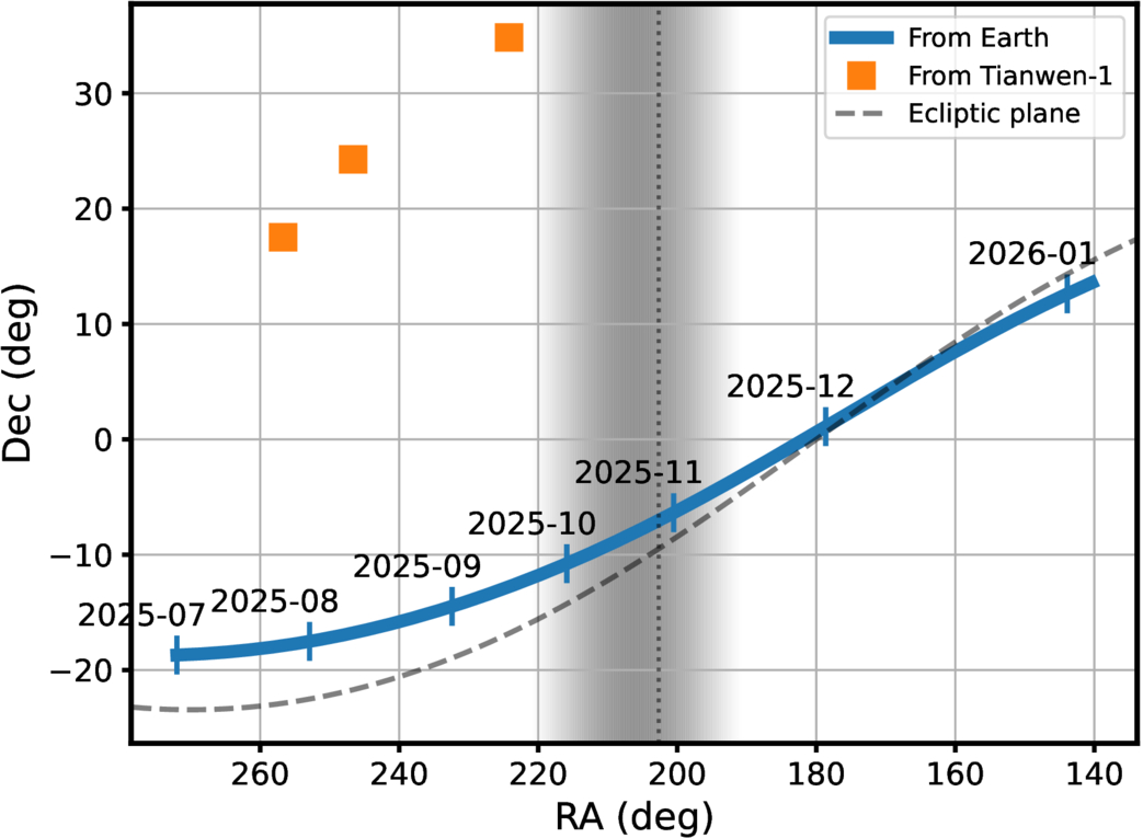
A plot showing that Earth-based observations could only get as best a 20-degree out-of-plane view, while Mars-based observations could get up to nearly 40.

3I/ATLAS’s path across the sky as seen from Earth versus the clearer line of sight from Mars. The shaded region represents the times where the comet was too close to the Sun for viewing. [Xin Ren et al. 2026]

Unfortunately for astronomers, 3I/ATLAS didn’t make it easy for them to study the shape of its coma. Thanks to a cosmic coincidence, the interstellar visitor was traveling almost perfectly within the plane of our solar system, and Earthbound observers were often limited to an edge-on view of its tail. Even worse, 3I/ATLAS looped around the back of the Sun from our perspective, meaning no one on the planet could observe the comet for a few weeks in the fall. This led a group of astronomers to consider their assets that are farther from home.

Better View from Mars

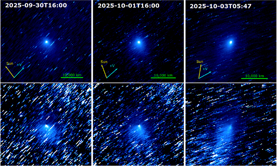
The Tianwen-1 spacecraft, which entered Martian orbit in early 2021 and has been diligently mapping the Red Planet ever since, has a high-resolution camera that’s normally pointed at the planet’s surface. By spinning the spacecraft around, a team of researchers led by Xin Ren (National Astronomical Observatories, Chinese Academy of Sciences) repurposed the camera to act as a small telescope when 3I/ATLAS flew by. In another cosmic coincidence, 3I/ATLAS happened to pass very near Mars last fall, and this close approach gave Tianwen-1 a great out-of-plane view of the coma. The orbiter managed to capture 57 images of 3I/ATLAS over three days last fall, representing China’s first-ever observations of an object from an asset in deep space.

Multi-panel photographs of a comet against a background of streaked stars.

Stacked images of 3I/ATLAS from the Tianwen-1 orbiter across three epochs; the tail’s apparent shape shifts as the viewing geometry changes. Click to enlarge. [Xin Ren et al. 2026]

The team took full advantage of the great view and leveraged the spacecraft’s unique perspective to extract some intriguing results. By tracking how the gentle pressure of sunlight nudged the escaping grains, the researchers found that the coma is dominated by surprisingly large dust. With an average size of hundreds of microns across, the dust is more like coarse sand than smoke, and they found that it ambles away from the comet at just 3–10 meters per second. All told, 3I/ATLAS was shedding dust at roughly 1,000 kilograms every second. The big grains may be a fingerprint of a cold, distant birthplace: models suggest such grains collect in the frigid outer reaches of planet-forming disks, hinting that 3I/ATLAS was forged far from its parent star before being flung into the dark.

As new surveys begin to turn up interstellar interlopers more often, this improvised observation makes a tidy point: the spacecraft already scattered across the solar system can double as a fleet of opportunistic comet-watchers, each offering a view we simply can’t get from home.

Citation

“Interstellar Object 3I/ATLAS Observed from Mars by China’s Tianwen-1 Spacecraft,” Xin Ren et al 2026 ApJL 1003 L10. doi:10.3847/2041-8213/ae61b3

The post Courtside Seats on Mars appeared first on AAS Nova.

  •  

The First Starspot Spectrum Revealed by JWST

M-dwarf star with starspots

Editor’s Note: Astrobites is a graduate-student-run organization that digests astrophysical literature for undergraduate students. As part of the partnership between the AAS and astrobites, we occasionally repost astrobites content here at AAS Nova. We hope you enjoy this post from astrobites; the original can be viewed at astrobites.org.

Title: A Panchromatic JWST Spectrum of a Giant Starspot on the Fully Convective M Dwarf TOI-3884
Authors: C. A. Murray et al.
First Author’s Institution: University of Colorado Boulder
Status: Published in ApJ

We often picture stars as smooth, glowing spheres, as if they’ve been run through an Instagram filter. But real stars have spots: cooler, darker regions on a star’s surface caused by strong magnetic fields.

Annoyingly, these spots can seriously interfere with how we study exoplanet atmospheres.

How to Probe a Planetary Atmosphere

Planetary atmospheres are often probed through transmission spectroscopy. When a planet transits its star, some starlight passes through the planet’s atmosphere before reaching us. We can distinguish the light that has passed through the planet’s atmosphere by comparing the star’s light in transit versus out of transit. In doing so, we can isolate the atmospheric spectrum and look for absorption features of species like water or oxygen.

Easy, right?

How Starspots Get in the Way

Things get more complicated once we stop thinking of the star as if it’s been smoothed out by an Instagram filter. Starspots are cooler than the surrounding stellar surface, which means they emit a different spectrum. They are also constantly changing: new spots can form, old ones can disappear, and the star’s rotation carries them in and out of view. This changes things.

First of all, your star’s spectrum changes over time, which could mean that the star’s spectrum out of transit is not the same as the star’s spectrum during transit. On the other hand, the planet may transit across a starspot instead of a “normal” stellar region. In this case, the light we measure during the transit is affected by the spot, and it is no longer accurate to directly compare it with the overall stellar light outside the transit.

Ultimately, absorption features that we thought were from the planetary atmosphere could actually be coming from starspot contamination instead.

Starspot Models: Our Solution?

To deal with this, astronomers build starspot models, where they vary the spots in terms of the following:

  • The surface covering fraction: this parameter tells us how much of the stellar surface is covered in spots
  • The temperature contrast: this parameter tells us how much cooler (in ratio) the spot is compared to the rest of the stellar surface, and by proxy how much dimmer

These models are promising, but how do we know that we have chosen the right parameters?

A Unique Laboratory: TOI-3884

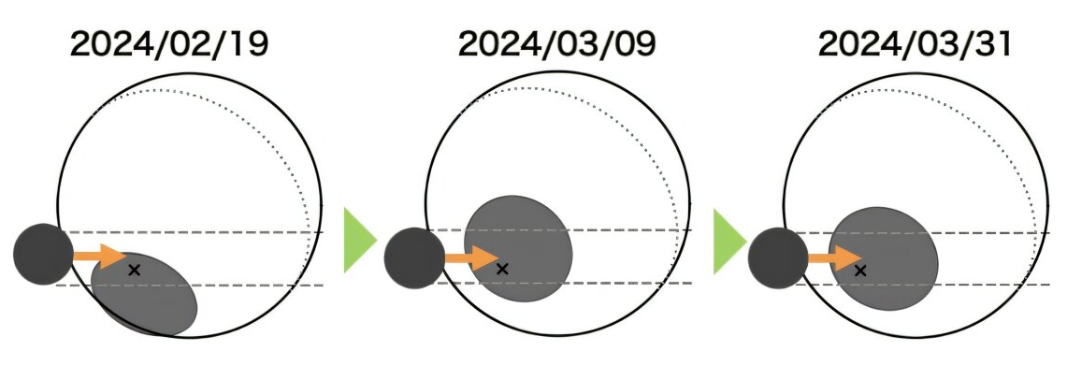
The TOI-3884 system is a unique laboratory for testing our starspot models. As seen in Figure 1, it has very convenient starspot geometry, with a large starspot located close to its pole. On top of that, we observe this star almost completely pole-on, which means that we always see this starspot, no matter how much the star rotates. To top this all off, the star hosts a close-in planet, which orbits the star from pole to pole.

Illustration of the TOI-3884 system

Figure 1: Illustration of the TOI-3884 system. The pole (and rotation axis) of the star is indicated with a black “x,” indicating that we see the star almost pole-on. The polar starspot is indicated in grey, and the transiting planet TOI-3884b is indicated in black. Different dates are shown, illustrating how the system evolves over the span of a few weeks. [Adapted from Mori et al. 2025]

The planet transits the star, and as it does so, it always passes over the polar starspot. This gives us a rare opportunity to probe the spectrum of a starspot. Similar to how we can use normal in/out of transit observations to probe a planetary atmosphere, we can now compare the observations during/after a “starspot transit” to probe the starspot region. Today’s authors do exactly this using six different transit observations from JWST.

So… How Good Are Our Models?

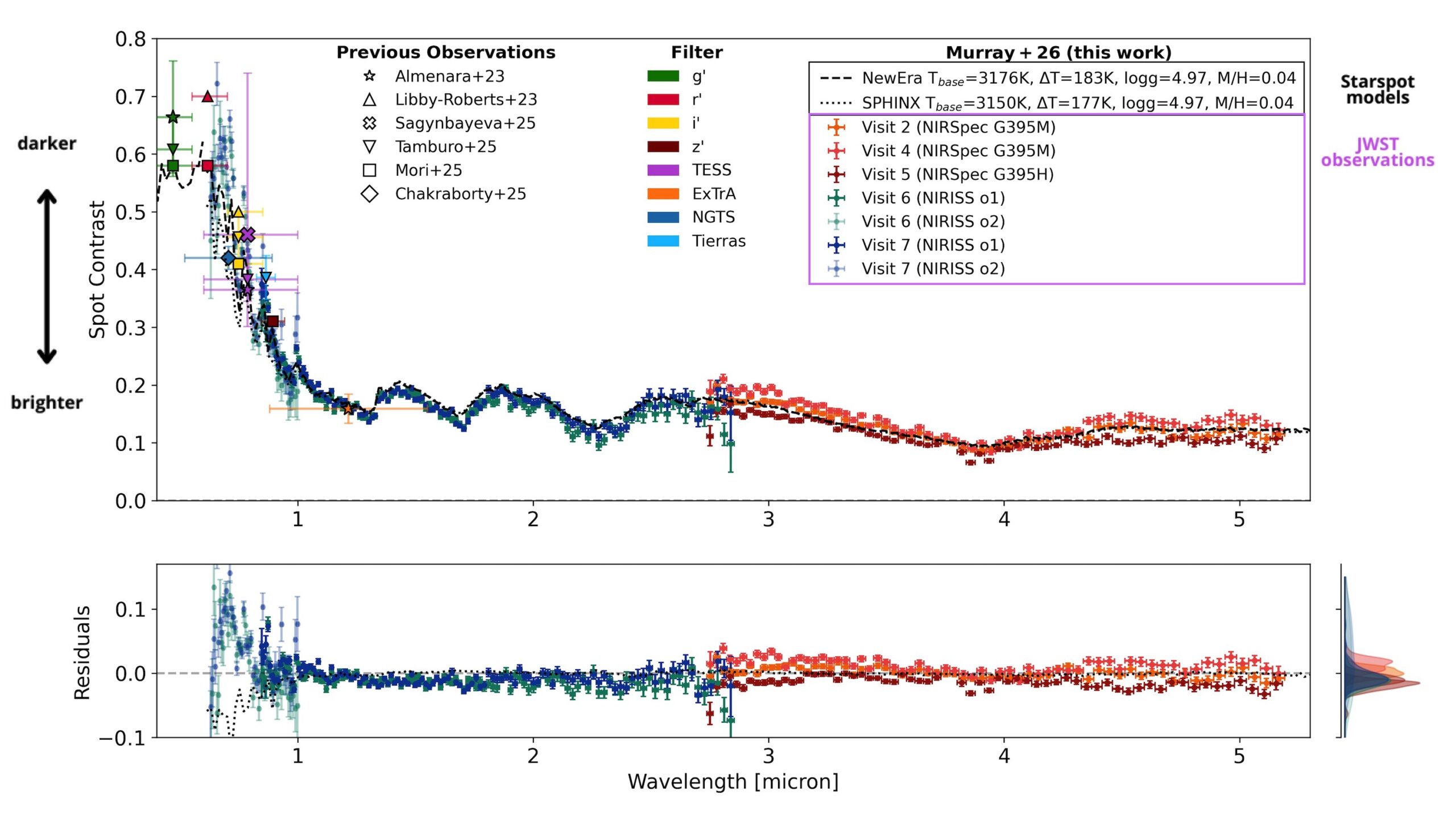
From the JWST observations, the authors extract a starspot spectrum for the first time. Figure 2 shows this as the spot contrast (how much dimmer the spot is than the surrounding stellar surface) plotted across different wavelengths. To see how well our models are doing, they compare this observed spectrum to two commonly used starspot models. The difference between the data and the models (the residual) is plotted in the lower panel.

spectrum of TOI-3884’s starspot.

Figure 2: The spectrum of TOI-3884’s starspot. The y-axis in the upper panel, the spot contrast, indicates how much dimmer the starspot is compared to the “normal” stellar surface. Different observations taken with JWST are indicated in different colored crosses, and other previous observations are overplotted in various other shapes. Model starspot spectra are shown in dashed or dotted black lines. The residuals between the model spectra and the JWST observations are shown in the bottom panel. [Adapted from Murray et al. 2026]

At wavelengths longer than about 1 micron, in the near-infrared regime, things look good! The residuals stay small, meaning the models do a solid job reproducing the observations. But move left into shorter wavelengths, in the optical regime, and the agreement quickly falls apart. The residuals grow, and it becomes clear that the models are missing something.

There’s still work to be done before we can confidently probe planetary atmospheres at optical wavelengths without worrying about stellar contamination, and this observed starspot spectrum provides a unique benchmark to test future starspot models. For now, the near-infrared remains a safer and more reliable window for planet atmosphere studies.

Original astrobite edited by Natalie Price.

About the author, Elise Koo:

I’m a PhD student at the University of Amsterdam, working to detect magnetic interactions between stars and their planets using radio and spectroscopic observations. Outside of research, I like to try out a variety of sports.

The post The First Starspot Spectrum Revealed by JWST appeared first on AAS Nova.

  •  

Life on the (Red) Edge

Earth in visible and near-infrared light

Editor’s Note: Astrobites is a graduate-student-run organization that digests astrophysical literature for undergraduate students. As part of the partnership between the AAS and astrobites, we occasionally repost astrobites content here at AAS Nova. We hope you enjoy this post from astrobites; the original can be viewed at astrobites.org.

Title: Retrieving the Red Edge on Earth-Like Planets with Heterogeneous Clouds and Surfaces
Authors: Zachary Burr et al.
First Author’s Institution: Jet Propulsion Laboratory; ETH Zurich
Status: Published in ApJ

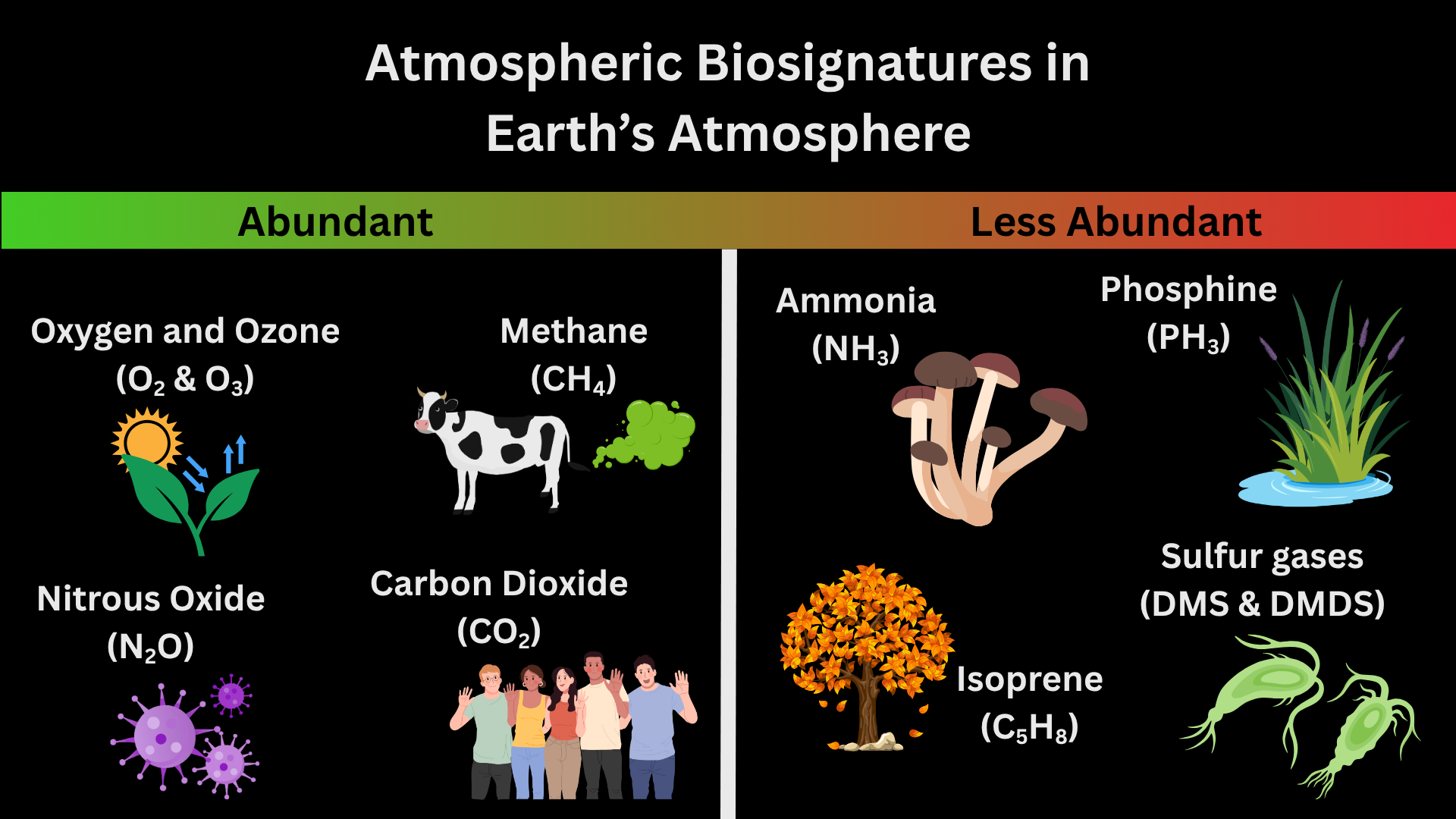
In the next 25 years, astronomers could find signs of life on other planets with the launch of the Habitable Worlds Observatory. Atmospheric signs of life, known as atmospheric biosignatures, are how astronomers currently search for life on other planets. Figure 1 shows examples of atmospheric biosignatures with pictures of each chemical’s origin on Earth. Before E.T. can phone home, though, we have to understand what chemicals make up a planet’s atmosphere. To do this, astronomers can use spectroscopy to observe a planet’s atmosphere in different wavelengths and measure the types and quantities of chemicals present.

biosignatures in Earth's atmosphere

Figure 1: Atmospheric biosignatures present in Earth’s atmosphere. More abundant biosignatures include oxygen and ozone (byproducts of photosynthesis in plants and bacteria) and nitrous oxide (byproduct of bacteria that don’t need oxygen to survive). Less abundant biosignatures include isoprene (released from the breakdown of leaves that have fallen from trees) and sulfur gases (byproducts of cyanobacteria). [Kaz Gary]

There are many ways to observe the spectrum of a planet, but the one you’re probably most familiar with is transmission spectroscopy. You can learn more about transmission spectroscopy of exoplanet atmospheres and how to model transmission spectra with these bites: 1, 2, 3. However, all of the current techniques for exoplanet spectroscopy (including transmission spectroscopy) measure the star’s light and how the planet affects the star’s light. This means it’s heavily dependent on how we model the star’s light to indirectly observe the planet’s light. The only way to take the spectrum of a planet directly is with direct imaging: the technique that the future Habitable Worlds Observatory will use to find signs of life in planetary spectra.

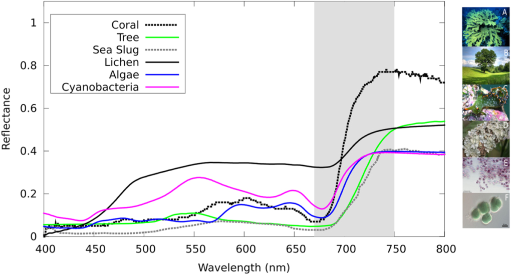
But are atmospheric biosignatures the only way to tell if life exists on other planets? Short answer: absolutely not. Let’s take Earth as an example. If we imagine Earth as a directly imaged exoplanet and take spectra of the light it reflects, you’ll find that around near-infrared wavelengths (~700 nanometers or just past the red part of the visible light spectrum), the light reflected off of Earth increases sharply. This sharp increase is called the vegetation red edge and is caused by plant and ocean life on Earth’s surface as shown in Figure 2. This is made possible because chlorophyll (the thing that makes plants green) absorbs nearly all visible light but reflects near-infrared light. The vegetation red edge is an example of a surface biosignature. In today’s article, the authors determine if the vegetation red edge will be visible in spectra of Earth-like exoplanets!

Spectra of different sources of the vegetation red edge

Figure 2: Spectra of different sources of the vegetation red edge on Earth. The vegetation red edge is highlighted in gray where the spectra rapidly increase and then level off beyond the visible light part of the spectrum. Each color represents a different source with pictures of each source on the right-hand side of the plot. [O’Malley-James and Kaltenegger 2019]

Snapshots

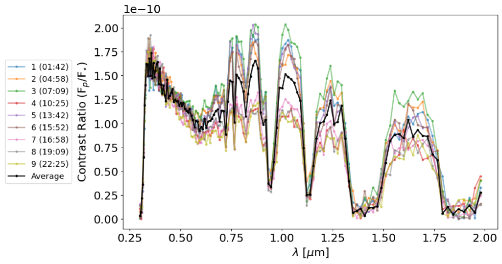
Planets rotate; that’s how we have morning, noon, and night in 24 hours guaranteed. This means that different parts of the surface will be visible at different times when we take spectra. Sometimes, we may see more ocean than land, other times not. To determine if the vegetation red edge would be visible at all points in Earth’s day, the authors simulated nine different spectra of modern-day Earth representing nine snapshots of Earth’s rotation. Additionally, they also simulated a time-averaged spectrum that shows an entire Earth day in one snapshot without the time variability. These spectra are shown in Figure 3.

Spectra of a directly imaged modern-day Earth at nine different times in its rotation

Figure 3: Spectra of a directly imaged modern-day Earth at nine different times in its rotation. The y-axis is the ratio of the planet’s signal to the star’s signal and the x-axis is wavelength in microns. Each color represents a time in UTC and the black curve represents the time-averaged spectrum. [Burr et al. 2026]

The authors then run retrieval models on all nine spectra to see if the vegetation red edge would be detectable in each spectrum, including the time-averaged one. Retrieval models take into account characteristics of the planet that would affect how light moves through its atmosphere, such as the atmospheric chemicals present and the surface gravity. They then use this information to generate possible spectral models that could fit the data. The best-fit model allows astronomers to infer what the atmosphere is made of and properties of the planet such as surface gravity. Because we are looking at Earth in visible light, much of the light from the planet is reflected. Typically, models of Earth-like planets in visible wavelengths only include atmospheric albedo: the measure of how reflective a planet’s atmosphere is. However, surface biosignatures can also be reflective as shown by the vegetation red edge. The authors use this to their advantage and introduce a surface albedo into their model that changes with the amount of desert, vegetation, and ocean visible on Earth’s surface at that time. They then further divide the nine spectra into three different types based upon the visible surface: majority land; 50% land, 50% ocean; and majority ocean. Check out the article online to see a cool animation of the Earth rotating and how the spectrum looks different at each time!

Arr! There Be… Vegetables?

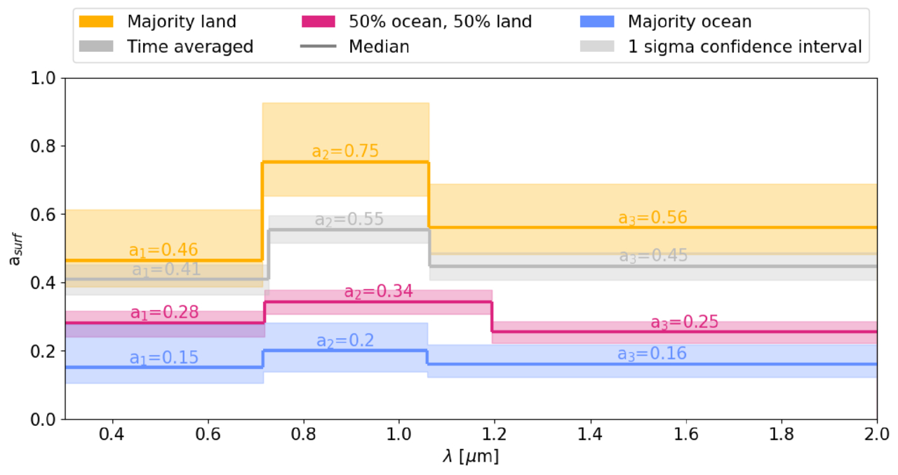
After running the models, the authors were able to detect a sharp increase in the surface albedo value in every spectrum, including the time-averaged one. This result is shown in Figure 4. The authors take this result one step further in order to validate that the vegetation red edge is actually a result of surface variation of vegetation. They re-run models on each of their spectra but instead include a constant surface albedo instead of a time-varying one. This resulted in incorrectly measured radii, chemicals, and surface gravity in nearly all of the models. Without the vegetation red edge and surface features, the models could not accurately determine if life was present on Earth.

Retrieved surface albedos for the nine time-varying spectra

Figure 4: Retrieved surface albedos for the nine time-varying spectra. The surface albedo is broken down into three different values (a₁, a₂, a₃). Each of these values represents a change in the surface albedo at different wavelengths (i.e., how reflective the surface is at three different wavelengths). The nine spectra were broken down by the amount of surface that was visible at that time and color-coded for each category. The time-averaged spectrum is shown in gray. Each category of spectra was able to retrieve an increase in reflected light from the surface at vegetation red edge wavelengths. The spectra that had the majority land visible have the biggest increase in the surface albedo. This makes sense since the amount of visible vegetation is the largest with majority-land planets. [Burr et al. 2026]

For the first time (to the author’s knowledge), the vegetation red edge has been shown to be a promising and observable biosignature in Earth-like atmospheres. This study has also laid the groundwork for future work on other surface biosignatures and their potential impact on spectra of habitable planets. Confirming signs of life in multiple different ways, both on the surface and in the atmosphere, will finally allow astronomers to say we are not alone in the universe. In fact, life likes to live on the (red) edge!

Original astrobite edited by Madison VanWyngarden.

About the author, Kaz Gary:

I am a fourth-year PhD candidate at The Ohio State University with a passion for planets. My current work focuses on modeling exoplanet observations for the Habitable Worlds Observatory and understanding planetary atmospheres. Outside of research, I help develop planetarium shows and love all forms of science communication. In my free time, I enjoy playing tabletop RPGs, painting, watching terrible reality TV, and hanging out with my pet hedgehog.

The post Life on the (Red) Edge appeared first on AAS Nova.

  •  

Playing Pool with Planets

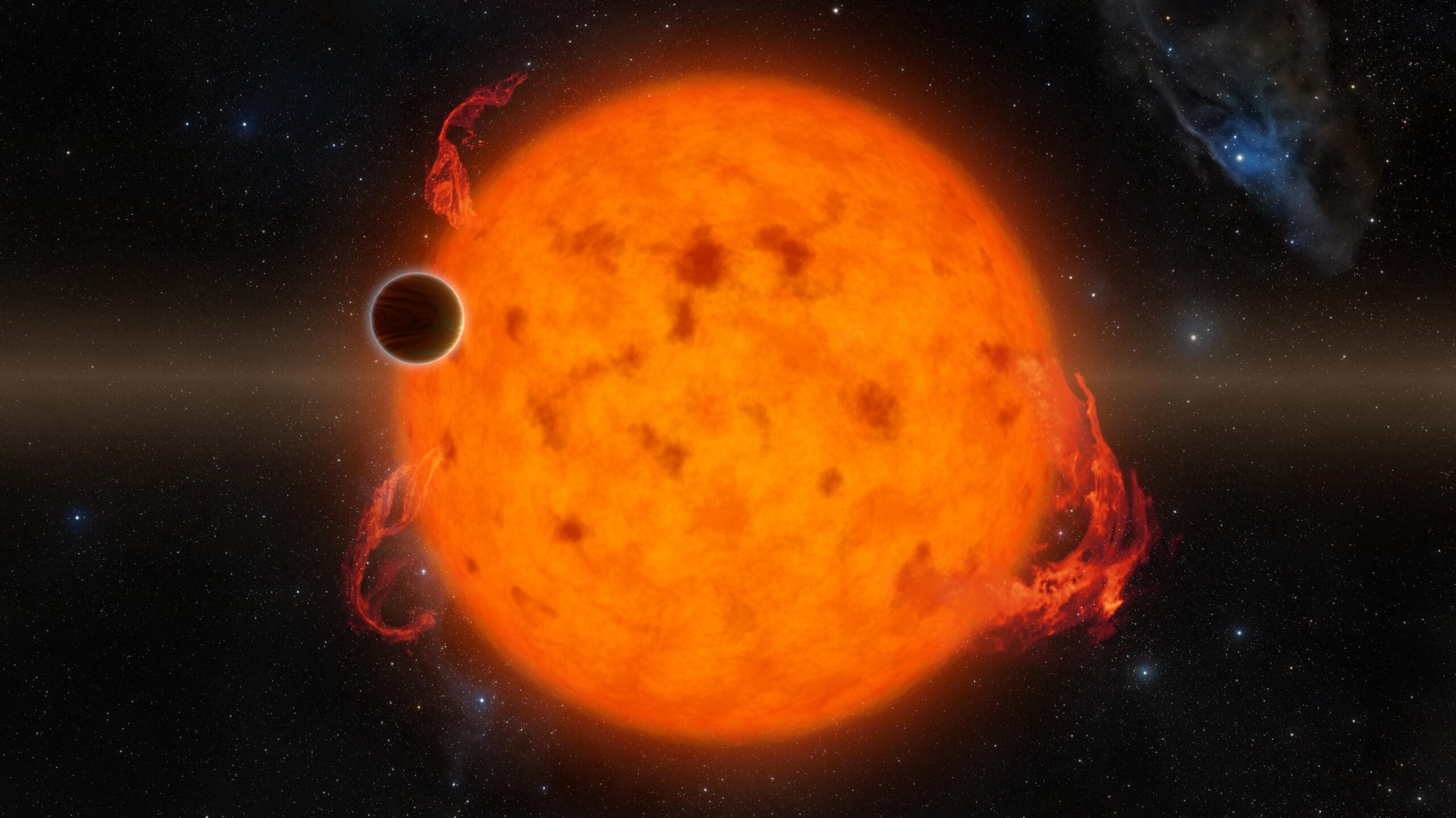
artist's impression of hot Jupiter exoplanets

Each Jupiter-size planet in the galaxy falls into one of three distinct categories: hot, warm, or cold. A new study suggests that despite the apparent differences between these populations, they may have all formed from the same underlying dynamical process: a game of pool played at planetary scales.

A Diversity of Jupiters

Though our solar system has only one Jupiter-size planet, elsewhere in the galaxy we have found three different species of these massive gas giants. Cold Jupiters closely resemble their namesake and orbit far from their host stars; hot Jupiters are the opposite and are found whipping around their stars on extremely close-in orbits. In between these are the warm Jupiters, which tend to orbit in the intermediate space between 0.1 and 1.0 au.

A rendering of a star with lots of spots and flares with a planet in the foreground.

An artist’s depiction of a hot Jupiter. These planets orbit extremely close to their host stars, but likely got to their locations by scattering inward from more distant orbits. [NASA/JPL-Caltech]

Though these three populations are defined by their orbital distances, they differ from each other in other ways as well. For example, hot Jupiters almost never have nearby companions; if there are any other planets circling the same star, they’re usually far-out cold Jupiters. They can also orbit in pretty much any direction, including opposite the direction of their star’s spin, and are usually on perfectly circular orbits. In contrast, warm Jupiters often have friends nearby, are much more aligned with their stars’ spins, and can have modest eccentricities.

Given these differences, it’s often thought that each of these populations arrived at its current location through different dynamical processes and that the history of the warm Jupiters is likely quite different from the history of the hot Jupiters. However, a new study led by Julia Esposito (Georgia Institute of Technology) has proposed an alternative view. Maybe these populations, though they appear different now, were all created by the same process: planet–planet scattering.

Virtual Planetary Billiards

A cartoon of Jupiters at different distances from the sun with labelled arrows flowing inwards and outwards from each.

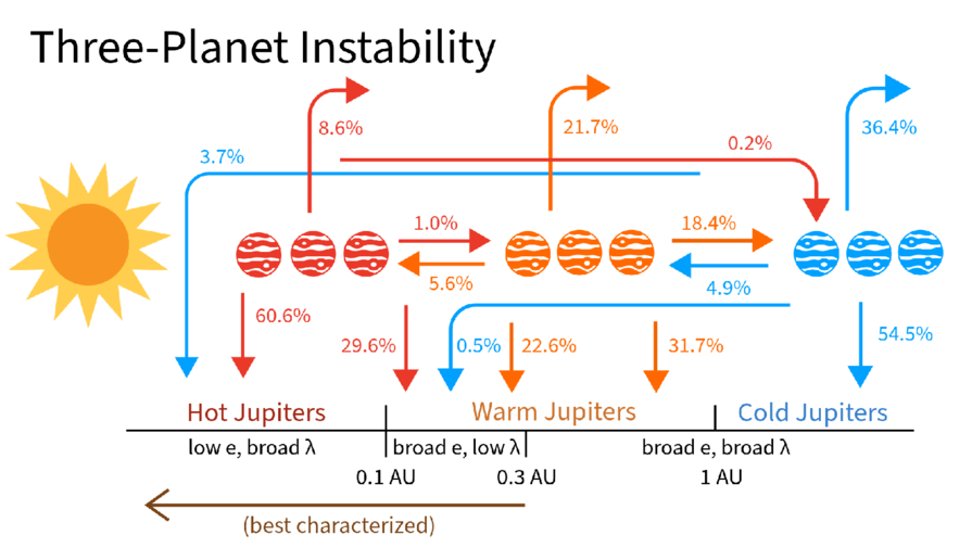
A schematic showing where different planets ended up as a function of where they scattered from during their evolution. Click to enlarge. [Esposito et al. 2026]

Esposito and collaborators set up 1,500 virtual planetary systems with three massive planets each, then simulated how the orbits evolved before probing the final configurations. In crucial contrast to previous simulation studies, the team initialized their Jupiters across a range of different distances and included the effects of tides sapping energy from orbits of planets that got too close to their host stars.

At the end of the simulation, the team surveyed the digital carnage. Almost every virtual system ended with only two planets after either ejecting one away from the star or having two planets collide. But, remarkably, the remaining two-planet systems looked tantalizingly similar to what we actually observe, with a mix of hot, warm, and cold Jupiters. Even more exciting, the end populations were highly correlated to where the violent scattering event took place.

For example, the warm Jupiters were almost all produced by “warm scattering” simulations, where the scattering took place between 0.1 and 1.0 au. The planets that survived the simulations and ended up as warm Jupiters matched all of the properties of the real warm Jupiter population: they had nearby companions, were moderately eccentric, and were mostly aligned with their stars. The hot Jupiters, meanwhile, were almost all produced by “cold scattering” events where the flybys happened far from the star and resulted in one planet hurtling inwards. These also matched all of the observed properties of real hot Jupiters.

The researchers concluded that planet–planet scattering can produce both the warm and hot Jupiter populations so long as you let the planets scatter from a variety of different distances. This exciting theoretical insight, if correct, would mean that astronomers could stop searching for different pathways to create each population. Happily, this model also provides testable predictions, and the authors lay out how the theory could be supported or disproven with additional data. Through virtual experiments like these, astronomers continue to build up an understanding of how the wide range of planetary architectures observed across the galaxy came to be.

Citation

“Unified Formation Channel of Hot and Warm Jupiters via Planet–Planet Scattering,” Julia Esposito et al 2026 ApJL 1003 L3. doi:10.3847/2041-8213/ae61b0

The post Playing Pool with Planets appeared first on AAS Nova.

  •  

I Spy with My Large Binocular Eyes: A Dusty Torus Around a Supermassive Black Hole?

NGC 4151

Editor’s Note: Astrobites is a graduate-student-run organization that digests astrophysical literature for undergraduate students. As part of the partnership between the AAS and astrobites, we occasionally repost astrobites content here at AAS Nova. We hope you enjoy this post from astrobites; the original can be viewed at astrobites.org.

Title: Shocks, Winds, and a Torus: The Large Binocular Telescope Interferometer (LBTI) Resolves the Active Nucleus of NGC 4151
Authors: Jacob W. Isbell et al.
First Author’s Institution: University of Arizona
Status: Published in ApJ

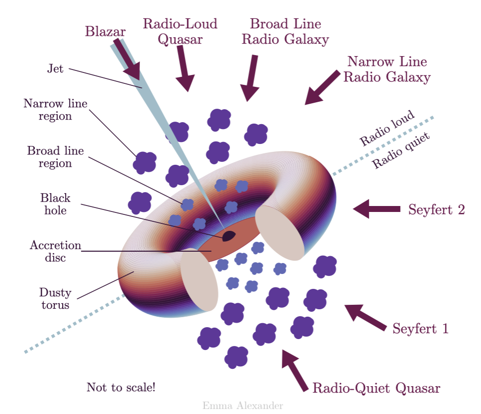
At the centre of nearly every galaxy lies a supermassive black hole that dominates this innermost region. Not only is there this millions-of-solar-masses dark beast, but usually too a whole bunch of stuff — stars, gas, dust, and more — which is often quite bright! When there is plenty of this material quite close to the black hole, we believe physics takes control to flatten it into a family of disk and toroidal structures in what we call the unified model of active galactic nuclei (AGNs; see Figure 1).

schematic of the unified model of active galactic nuclei

Figure 1: The unified model of AGNs asserts that there is an inner accretion disk, surrounded by a dusty torus that cohabitates with clouds moving at different velocities (the so-called broad and narrow line regions), and sometimes even relativistic jets extending from the accretion disk to galactic scales; you can read more about AGN structure in this Astrobites guide. [Emma Alexander; CC BY 4.0]

When astronomers look at different active galaxies (read: galaxies with active supermassive black holes at their core), we see a range of phenomenologies related to their brightness, spectra, morphologies, and more. The unified model of AGNs seeks to explain these different AGN appearances simultaneously by positing that they all have the same physical structure, and we are just viewing them from different angles, hence seeing different features.

The cores of AGNs are often imaged at the smallest scales (e.g., their accretion disks, viewed with interferometers like the Very Large Telescope Interferometer) and the largest scales (e.g., their relativistic jets, viewed with radio interferometers), but comparatively less effort has gone to directly observing the predicted dusty tori in the mid-infrared. That is exactly what today’s authors set out to do using the Large Binocular Telescope Interferometer (LBTI) — a pair of 8.4-metre-aperture mirrors separated by just over 14 metres and combined to simulate a telescope effectively 29 metres wide. This lets astronomers take direct images at a much higher resolution than a smaller-aperture telescope, and hence directly peer into the region around AGNs where this dusty torus should lie.

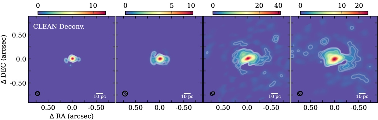
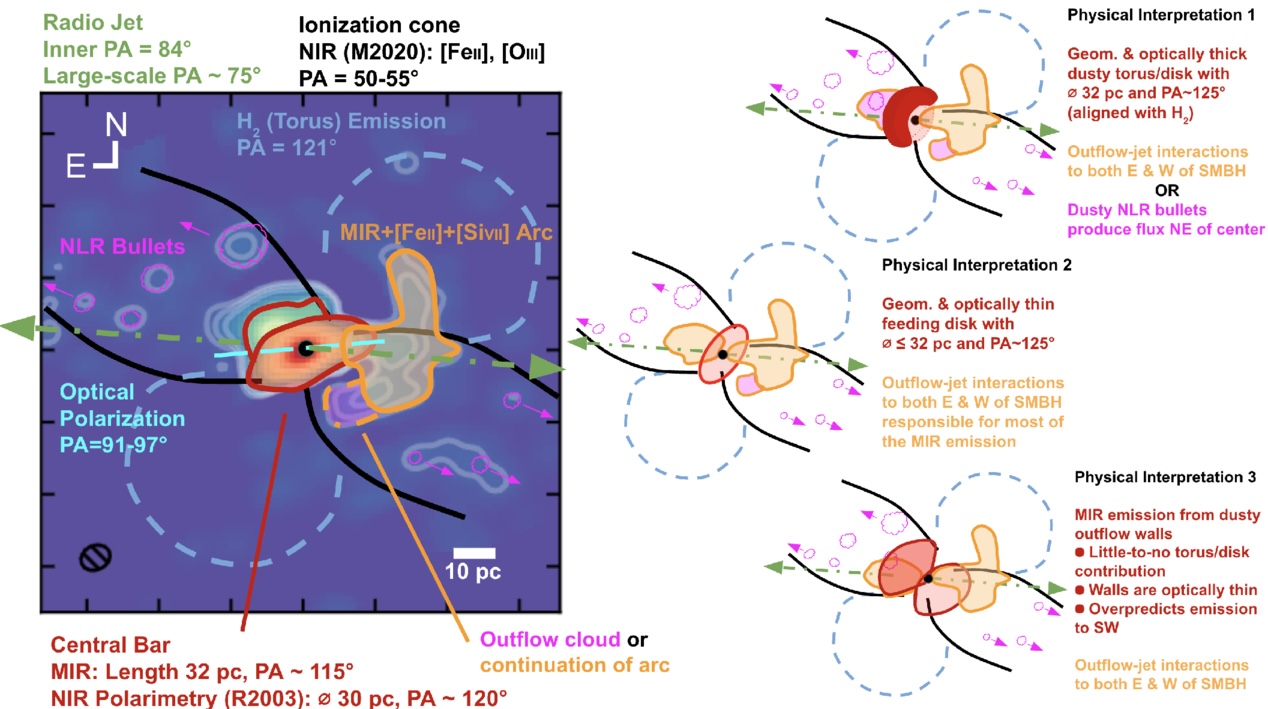
Today’s authors turn the LBTI towards NGC 4151, a medium-luminosity AGN. With the large effective aperture of the LBTI, they were able to resolve scales in the AGN region as small as 4.4–9.1 pc, about 14–30 light-years depending on the wavelength (see Figure 2), in the mid-infrared. These observations revealed warm dust emission in a complex structure around the central supermassive black hole. The authors note a central bar at all wavelengths, with a significant extension of cool dust arcing to the west (right in the image) and warmer dust localised to the centre (as evident by 3.7- and 4.8-micron emission only nearest to the supermassive black hole and its accretion disk).

deconvolved images of the AGN core of NGC 4151

Figure 2: The deconvolved images of the AGN core of NGC 4151 show a very bright central source (the innermost region around the supermassive black hole), as well as some complex surrounding structure particularly at long wavelengths. The interpreted morphology is described in Figure 3. These images are deconvolved, meaning that known optical effects are corrected for on the raw data to produce a sharper image. [Adapted from Isbell et al. 2026]

To explain the observed morphology in Figure 1, the authors compare three different interpretations based on this new high-resolution imagery together with the results of previous studies looking at other scales and the spectrum of the AGN core. Each interpretation is illustrated and briefed in Figure 3.
illustration of the different regions surrounding NGC 4151's black hole and potential interpretations for the observed morphology

Figure 3: Three interpretations of the observed morphology are presented by the authors. The left panel illustrates the different regions surrounding the supermassive black hole (together with the results of other studies cited in the article). The right panel shows the suggested interpretations explaining the morphology. [Isbell et al. 2026]

The first interpretation is in keeping with the unified model of AGNs: a geometrically and optically thick torus of dust surrounds the inner region. In this interpretation, the surface of the dusty torus re-radiates light from the accretion disk to produce most of the mid-infrared emission. Additional mid-infrared emission could come from localised concentrations of gas or interactions between the outflow and the jet. The authors immediately disfavour this explanation, as other studies have shown bright ionised emission at the location of the would-be torus, which is not expected if an optically thick torus were to be present. Hence, these new observations somewhat challenge the one “flavour” of the unified model of AGNs.

The second interpretation aligns with a different version of the unified model: one in which a geometrically thin disk replaces a thick torus around the AGN core. Provided the disk is optically thin too, the authors favour this approach as it is consistent with the geometry of ionised emission that worked against the first interpretation. While other studies suggest that this thin disk should be optically thick, this morphology is at least better aligned with what we see in other AGNs.

The third interpretation suggests that the emission comes from only the radiation pressure–driven wind emanating from the AGN core. The authors disfavour this explanation, citing previous radiative transfer simulations that show that the flux should fall off with distance from the core too quickly to be consistent with the observations.

No matter the interpretation, these LBTI observations are an important glimpse into the future of mid-infrared AGN studies that will be done with 30-metre-class telescopes (such as the European Southern Observatory’s Extremely Large Telescope). This article, together with the group’s similar study on NGC 1068, is challenging and refining an accepted view of AGN morphology — the consequences of which apply to galaxies near and far — and poses new questions perfect for sophisticated hydrodynamic and radiative simulations.

Original astrobite edited by Margaret Verrico.

About the author, Ryan White:

I am a first-year PhD student at Macquarie University in Australia, working mainly on binary/multiple systems with massive stars (Wolf–Rayets in particular!). Outside of study, I’m probably drinking coffee, baking, reading, or going for a run. You can also find me procrastinating on Bluesky @astroryan.bsky.social.

The post I Spy with My Large Binocular Eyes: A Dusty Torus Around a Supermassive Black Hole? appeared first on AAS Nova.

  •  

Hunting for Exomoons Around a Lonely Planet

illustration of an exoplanet and exomoon around a star

Editor’s Note: Astrobites is a graduate-student-run organization that digests astrophysical literature for undergraduate students. As part of the partnership between the AAS and astrobites, we occasionally repost astrobites content here at AAS Nova. We hope you enjoy this post from astrobites; the original can be viewed at astrobites.org.

Title: A Deep Search for Exomoons Around WISE 0855 with JWST
Authors: Mikayla J. Wilson et al.
First Author’s Institution: University of California, Santa Cruz
Status: Published in AJ

The “Moon”-umental Question

The solar system hosts hundreds of moons, ranging from volcanic worlds like Io around Jupiter, to icy objects like Enceladus around Saturn, to captured objects like Neptune’s retrograde moon Triton. Moons are essential to our model of how the solar system formed and also offer some of the best chances we have for finding life beyond Earth.

Astronomers also expect exomoons, or moons orbiting planets outside the solar system, to be abundant around other giant exoplanets. But how common are exomoons? How do they compare to the moons in our solar system?

In order to begin answering those questions, we must first detect an exomoon, which has proved difficult despite decades of searching by astronomers. Fortunately, JWST presents a new opportunity to uncover the exomoon population by looking at lonely free-floating planets as they drift through space.

Why Free-Floating Planets?

One proposed method for searching for exomoons is by looking for their transits in front of their host planets, characterized by the dips in brightness of the planet as the moon passes in front, blocking the planet’s light. Looking for exomoon transits around planets orbiting stars is quite difficult, as the bright starlight can easily drown out the small signals of exomoon transits. Free-floating planets solve this issue by removing the star entirely, increasing our sensitivity to such detections. (See this bite for a good review.)

The authors of today’s article directed the exomoon hunt towards the free-floating WISE J085510.83-071442.5 (or WISE 0855). It has the prestige of being the coldest known brown dwarf (250–285K) while also sitting at a relatively low mass (3–10 Jupiter masses). Notably, it is also one of our closest neighbors at a distance of only 7.4 light-years, making it ideal for high-precision observations despite its faintness. Even though brown dwarfs are technically distinct from planets, the authors opt to refer to companions around WISE 0855 as moons given WISE 0855’s “planetary-mass” status. (It’s complicated…)

Repurposing JWST Data… for Moons!

The JWST observations used in this study contain 11 hours of near-infrared (2.87–5.27 microns) time-series spectra originally intended to study water clouds and weather on WISE 0855. Time-series brightness monitoring can also be used for transit searches, which the authors take advantage of.

One complication is that WISE 0855 is variable, meaning its intrinsic brightness changes over time. Variability is likely driven by clouds and other dynamic processes within its atmosphere. So how do the authors distinguish between a passing moon and a turbulent atmosphere? The key idea is that variability is wavelength dependent, meaning that the brightness of WISE 0855 will fluctuate differently depending on the observed wavelength. In contrast, transits are “gray,” meaning that the same amount of light is blocked at all wavelengths, producing a consistent feature across the entire spectrum.

Finding Moons with Statistics!

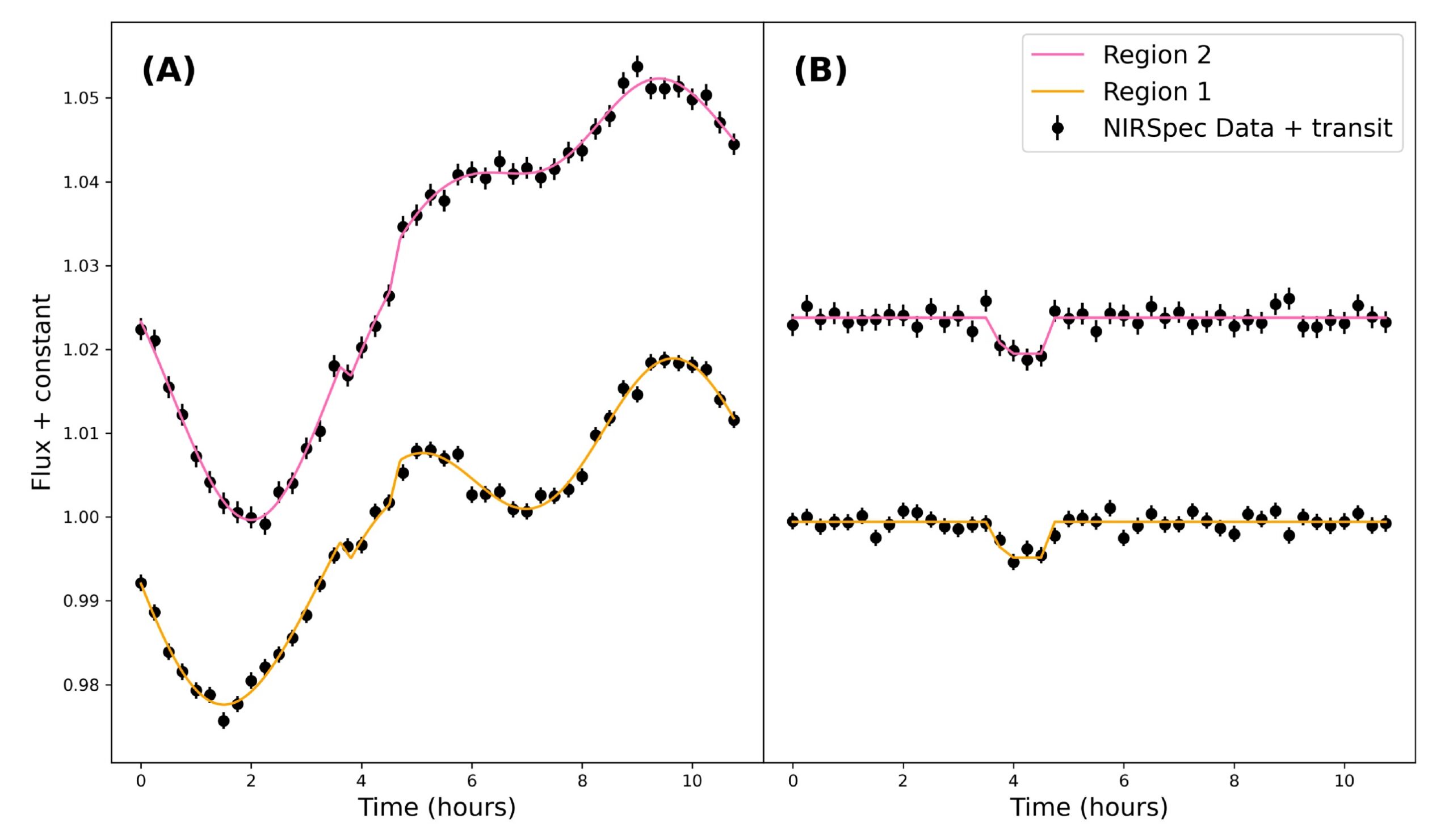
The authors apply this idea and pick out two wavelength regions of WISE 0855’s spectrum that contain two distinct variability patterns, which should both contain an identical moon transit signal (if present). They then generate a light curve (how brightness changes over time) for these two regions (see Fig. 1).

WISE 0855 light curves

Figure 1: (A) Light curves from two selected wavelength regions of WISE 0855’s spectrum with injected transit signals. Also plotted is the best-fit Gaussian processes + transit model for the two light curves. (B) Light curve data after subtracting the Gaussian processes portion of the best-fit model, revealing the example injected transit signals. [Wilson et al. 2025]

To appropriately model the variability, the authors employ Gaussian processes, a flexible tool that can model complex, quasi-periodic signals like atmospheric variability. They compare fits from two types of models:
  • Gaussian processes–only model: Assumes that all observed variability is intrinsic to the planet itself
  • Gaussian processes + transit model: Includes a simple trapezoidal exomoon transit signal that is simultaneously fit in both light curves

Using Bayesian evidence (a measure of how well each model explains the data), they determined which model was favored. So, what do they find?

The Bad News and the Good News

Based on Bayesian evidence, the authors conclude that there are no statistically significant detections of exomoons in the data. The results suggest very weak evidence for a ~0.53-Earth-radius moon at a wide separation from WISE 0855 — an unlikely scenario given that transit probability decreases at greater separations (and therefore longer orbital periods).

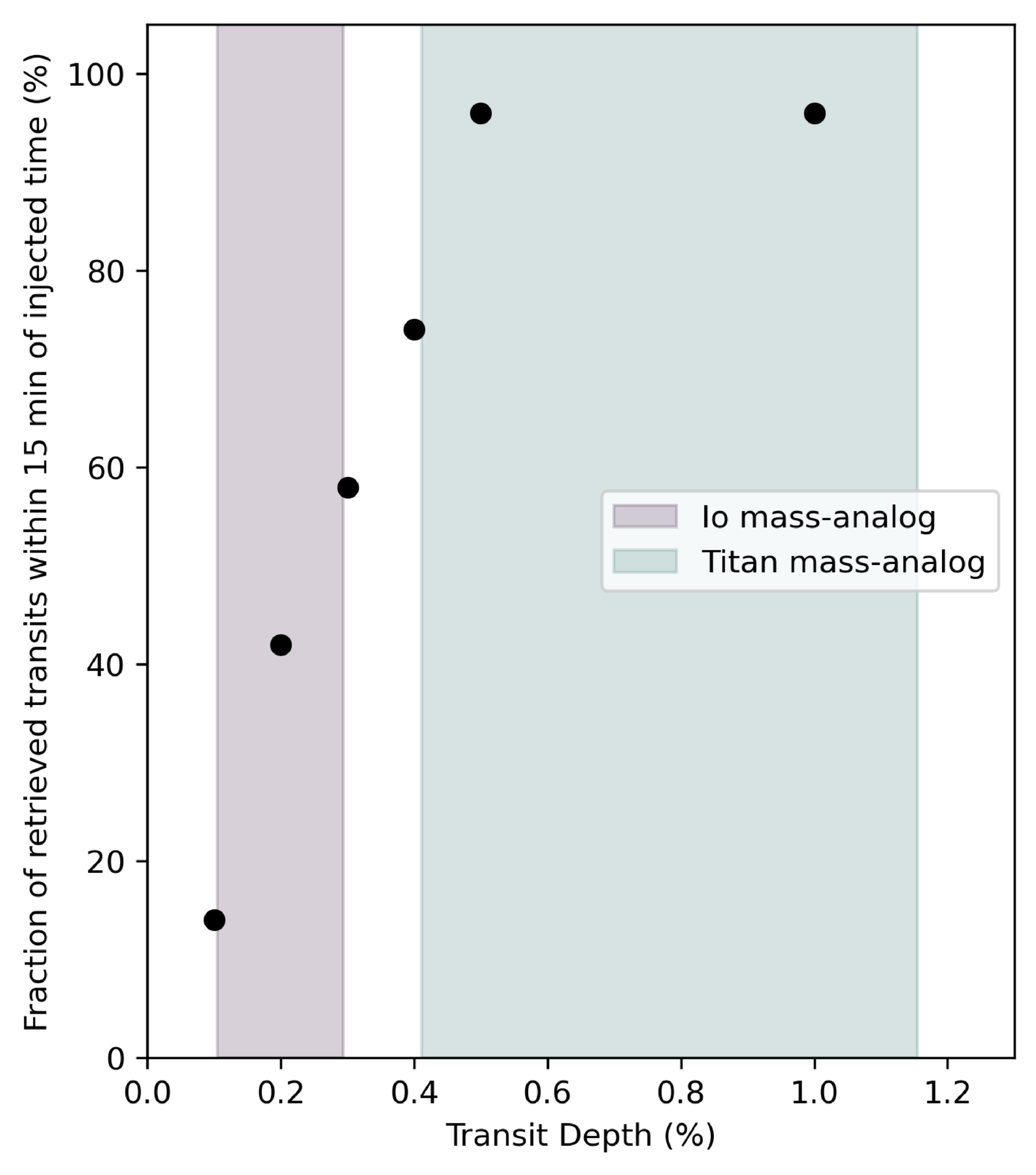
Yet, the study goes further: What kinds of moons is JWST able to detect, if any? To answer this, the authors performed injection and recovery tests, where they injected artificial transit signals of varying depths (exomoon sizes) into the data and tested how well their models were able to recover them (results shown in Fig. 2). They find that JWST is capable of detecting 96% of transits with depths ≥0.5%, equivalent to a Titan-like moon. Smaller Io-like moons were also detectable more than half of the time. This means that if a Titan analog had actually transited during these observations, we would almost certainly have seen it!

plot of successful detections of injected transit signals

Figure 2: Results showing the number of successful detections for the transit injection and recovery tests. Fifty transit injections are done for transit depths of 1%, 0.5%, 0.4%, 0.3%, 0.2%, and 0.1%. The transit depths represent different exomoon sizes, with the shaded regions representing Io-like and Titan-like moons. [Wilson et al. 2025]

JWST will continue to gather more time-series data of free-floating planets, brown dwarfs, and directly imaged exoplanets, each providing a new opportunity to help us better understand the moon population outside of our solar system. We’re still waiting for the first confirmed exomoon, but when that transit finally happens, we know that JWST will be ready.

Original astrobite edited by Kelsie Taylor.

About the author, Jared Bull:

I am a 2nd-year PhD student at Johns Hopkins University. I study brown dwarf variability and am interested in using time-series observations to uncover dynamic processes within their atmospheres. In my free time I like to read, cook, and do astrophotography.

The post Hunting for Exomoons Around a Lonely Planet appeared first on AAS Nova.

  •  

A New View of the Spectroscopic Universe

A photograph of a telescope opened at dusk.

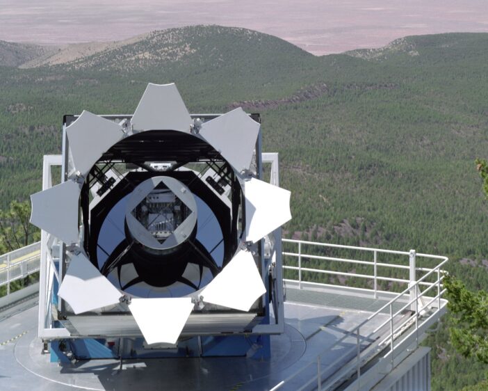
The Sloan Digital Sky Survey (SDSS) fundamentally changed the way modern astronomy research is done. This “grand and bold thing” is not frozen in a museum exhibit, however: instead, the SDSS telescopes and team have continued to iterate. The collaboration recently described the fifth generation of this groundbreaking survey in The Astronomical Journal.

Roots in History

Astronomy is now without question a “big data” science. While a lucky few researchers still occasionally travel to distant mountaintops to sojourn with the stars, most astronomers who can describe their work as “observational” rarely ever leave their laptops. Petabytes of historical data, including images, spectra, enormous simulation archives, and more, are available the instant one’s fingers touch a keyboard. As a result, the speed of discovery has increased exponentially, and the barriers to cutting-edge research have dramatically shrunk.

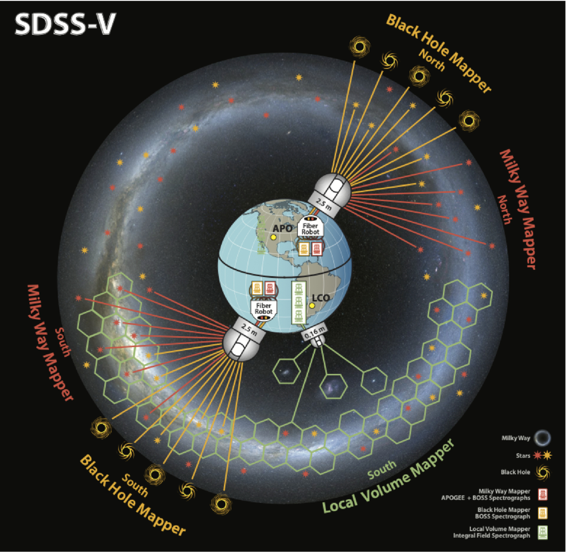
A cartoon of the Earth with three telescopes roughly geographically distributed as they are for the SDSS V survey.

A schematic of the SDSS-V survey facilities and targets. Click to enlarge. [Kollmeier et al. 2026]

While no paradigm shift can be pinned to an exact date, astronomy’s turn towards the data-rich era arguably began in 1998 when SDSS first began collecting data. This was among the first of the “industrial” surveys that observed large swaths of the sky with electronic detectors and used automated pipelines for bulk data processing. In the years since, larger robotic telescopes have begun to mimic the SDSS strategy of “mowing the sky.” The latest of these successors, which itself may usher in another paradigm shift in terms of data volume and availability, is the soon-to-begin Legacy Survey of Space and Time at the Vera C. Rubin Observatory.

While SDSS’s twin 2.5-meter telescopes (one in New Mexico and one in Chile, allowing the survey to observe the entire sky) are dwarfed by Rubin’s 8-meter mirror, there is still thrilling science to be done with these moderate-sized observatories. This is especially true after a series of upgrades to the spectrographs and thanks to a deep expertise in not only survey-style science, but also in project management and survey planning. In 2021, in the middle of COVID-19 delays and distancing requirements, the team began upgrades to their existing facilities and construction of a brand new telescope to kick off the latest survey, SDSS-V.

The Next Generation

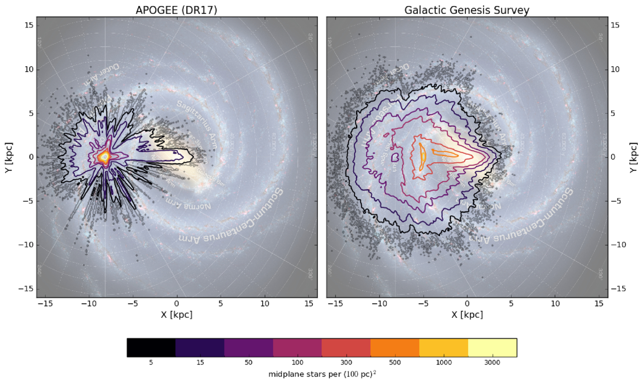
A two-panel figure showing top-down views of the milky way galaxy with different density contours overlaid.

The density of target stars for the SDSS-V survey compared to a previous spectroscopic survey. Click to enlarge. [Kollmeier et al. 2026]

In a wide-ranging publication that references not only astronomy research articles but also Plato, the Bhagavad Gita, an Egyptian tomb, and Tolstoy, the large collaboration describes that this latest survey is divided into three parts: the Milky Way Mapper, the Black Hole Mapper, and the Local Volume Mapper. The preexisting telescopes, which are outfitted with hundreds of tiny robots that can swivel fiber optic cables into place to collect spectra of up to 500 objects at a time, will handle the first two of these “mappers.” A brand-new facility in Chile that’s specifically designed to map the structure of nearby gas will handle the last mapper. Instead of aiming the fibers at a known star or galaxy, this telescope will instead collect a spectrum for every point across an area the size of the full Moon with every exposure.

By the end of the survey, SDSS-V will have collected optical and near-infrared spectra for roughly 6 million objects spread across the whole sky, as well as time-series spectra from about a million of these sources. This dataset, which is unprecedented in both its spatial and temporal coverage, will allow researchers to probe questions ranging from how quasars evolve over time to how commonly young stars have brown-dwarf companions. Long since SDSS initiated the era of industrial survey astronomy, this latest publication shows how the survey continues to lead the way.

Citation

“Sloan Digital Sky Survey. V. Pioneering Panoptic Spectroscopy,” Juna A. Kollmeier et al 2026 AJ 171 52. doi:10.3847/1538-3881/ae0576

The post A New View of the Spectroscopic Universe appeared first on AAS Nova.

  •  

Feed the Fire, Fade the Metals

galaxy cluster MACS J1149.5+2223

Editor’s Note: Astrobites is a graduate-student-run organization that digests astrophysical literature for undergraduate students. As part of the partnership between the AAS and astrobites, we occasionally repost astrobites content here at AAS Nova. We hope you enjoy this post from astrobites; the original can be viewed at astrobites.org.

Title: Metal-Poor Star-Forming Clumps in Cosmic Noon Galaxies: Evidence for Gas Inflow and Chemical Dilution Using JWST NIRISS
Authors: Vicente Estrada-Carpenter et al.
First Author’s Institution: Arizona State University
Status: Published in ApJ

If you want to reconstruct a galaxy’s life story, one of the best “fossil records” is its metallicity. In astronomy this refers to the abundance of elements heavier than helium, which are made in stars and returned to a galaxy’s gas through winds and supernovae. Over time, more star formation usually means more metals mixed into the gas.

Now zoom to Cosmic Noon (roughly when the universe was most actively forming stars). Many galaxies in this epoch look “clumpy”; their star formation is concentrated in several bright knots scattered across the disk. The big question is where those clumps come from. Do they form from the galaxy’s own gas via internal disk instabilities, or do they light up when fresh, metal-poor gas flows in and both fuels star formation and dilutes the local metallicity?

The authors try to answer that question with JWST by measuring the metallicity of each clump relative to its immediate surroundings, rather than comparing clumps to a single galaxy-wide number (which can be misleading if the galaxy has a metallicity gradient).

They use JWST/Near Infrared Imager and Slitless Spectrograph (NIRISS) slitless grism spectroscopy from the CAnadian NIRISS Unbiased Cluster Survey (CANUCS) to study 20 lensed galaxies at redshift 0.6 < z < 1.35. (Lensing effectively acts like a zoom lens, helping to resolve smaller structures.) They focus on emission lines that trace star-forming gas, especially Hα (a star formation tracer) and sulfur lines [SII] and [SIII] (needed for their metallicity method).

Slitless spectra come with a headache: because there is no slit, different parts of a galaxy can overlap in the dispersed image. To make reliable emission-line maps from slitless data, the authors use a forward-modeling code called Sleuth, which allows the continuum to vary across the galaxy.

The authors identify clumps using the Hα map together with rest-frame ultraviolet imaging because these tracers are sensitive to star formation on different timescales: Hα highlights gas ionized by the youngest massive stars, while ultraviolet light traces young stellar light over longer periods. As a result a clump can be bright in one and not the other, especially if dust is involved.

To estimate gas-phase metallicity, they use the “strong-line” method, which infers metallicity from ratios of bright emission lines calibrated using models and empirical samples. Their main diagnostic is S23 = ([SIII] + [SII]) / Hα. Because some line ratios also depend on the ionization state (how strongly the gas is being ionized by young stars), they also use the sulfur ratio S32 = [SIII]/[SII] as a check and iterate to a self-consistent solution.

So, Are Clumps Really Chemically Different from Their Surroundings?

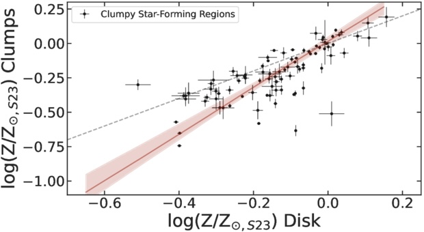
For each clump, the authors measure the metallicity inside the clump and compare it to an annulus just outside the clump (masking neighboring clumps to avoid mixing). When they plot “clump metallicity” versus “local disk metallicity,” most points fall below the 1-to-1 line, meaning the clumps are more metal poor than their surroundings (Figure 1). The mean offset is about 0.1 dex, which corresponds to roughly 20% dilution in the clump gas.

plot of gas-phase metallicity in star-forming clumps compared against metallicity of nearby disk regions

Figure 1: Each point compares a star-forming clump’s gas-phase metallicity to the metallicity of the nearby disk region immediately surrounding it. If clumps and disks had the same metallicity, they would lie on the dashed 1-to-1 line. Instead, most clumps sit below it, showing a typical ∼0.1 dex metallicity deficit, consistent with local chemical dilution. (The solid red line shows a best-fit linear trend to the clump measurement.) [Adapted from Estrada-Carpenter et al. 2025]

An extra wrinkle is that the galaxy medians hint at two populations: some galaxies have clumps with small offsets (near the 1-to-1 line), while others show larger offsets. The authors suggest this could mean two formation pathways, one dominated by internal gas reservoirs (smaller offsets) and another where inflow of metal-poor gas plays a bigger role (larger offsets). They are careful, though, as the sample is still small.

If inflow is really the driver, you should expect a link: the more strongly a clump is forming stars relative to its surroundings, the more diluted its metallicity should be. That is exactly what the authors find. The clumps that are most boosted in star formation are also the most metal diluted.

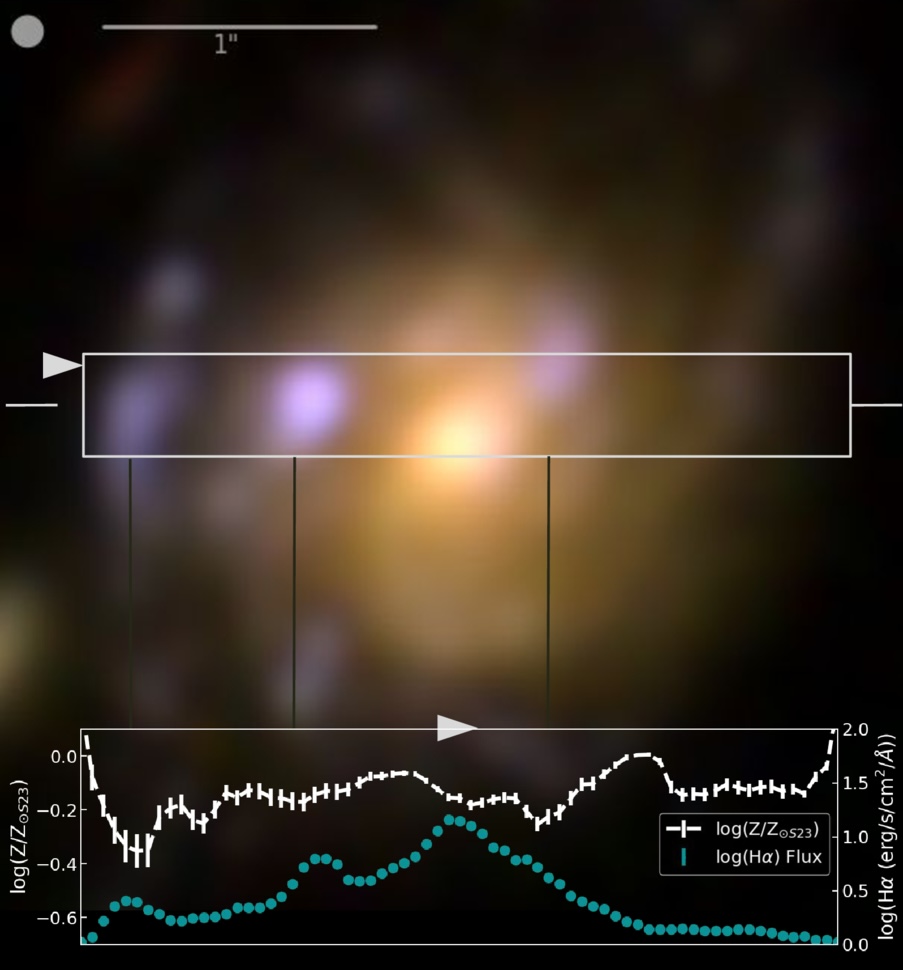
The article also emphasizes that clumps are not chemically uniform blobs. In at least one detailed example, the peaks in Hα (highest star formation) coincide with local minima in metallicity along a cut through the galaxy (Figure 2), suggesting internal star formation rate and metallicity gradients that reinforce the same story, intense star formation goes hand in hand with lower metallicity in the clump regions.

galaxy image showing spatial variation of H alpha and metallicity

Figure 2: Example galaxy from this study illustrating the clump-scale link between star formation and metallicity. The color image shows the galaxy with a rectangular strip marking the region used for a 1D cut. In the bottom panel, the turquoise line shows the Hα flux (a tracer of recent star formation), while the white line shows the metallicity along the same cut. Peaks in Hα flux line up with local dips in metallicity, showing that the brightest star-forming clumps are also the most chemically diluted compared to nearby regions. [Adapted from Estrada-Carpenter et al. 2025]

Are These Clumps Really “In Situ,” or Could They Be Small Satellites?

A reasonable alternative is that some clumps are actually small companion galaxies projected onto the disk. These could also look metal poor, because low-mass galaxies tend to be low metallicity. The authors look for evidence using face-on systems and find that more massive clumps tend to sit closer to galaxy centers, which is consistent with in-situ clumps that form in the disk and migrate inward, though it does not rule out satellites. They argue that kinematics from JWST/NIRSpec IFU will be needed for a definitive separation.

Why This Matters

Gas inflow, star formation, and feedback, together known as the baryon cycle, are key drivers of how galaxies grow. What this article adds is a spatially resolved view that compares each clump to its local environment, showing that regions of elevated star formation also tend to be locally metal poor. That pairing is hard to explain as a simple metallicity gradient or a galaxy-wide averaging effect, and it is exactly what you would expect if at least some clumps are being fueled by relatively metal-poor inflows. In short, these clumps may be snapshots of galaxies refueling in real time.

Original astrobite edited by Ryan White.

About the author, Niloofar Sharei:

I’m an astronomy PhD candidate at UC Riverside studying how galaxies grow through star-forming clumps. I track how these clumps emerge, evolve, and sometimes survive long enough to reshape their galaxies. When I’m not thinking about cosmic blobs, I’m reading, hiking, or listening to Bach.

The post Feed the Fire, Fade the Metals appeared first on AAS Nova.

  •  

The Oldest Starlight

illustration of stars in the early universe

Editor’s Note: Astrobites is a graduate-student-run organization that digests astrophysical literature for undergraduate students. As part of the partnership between the AAS and astrobites, we occasionally repost astrobites content here at AAS Nova. We hope you enjoy this post from astrobites; the original can be viewed at astrobites.org.

Title: Hunting for the First Explosions at the High-Redshift Frontier
Authors: Junehyoung Jeon et al.
First Author’s Institution: The University of Texas at Austin
Status: Published in ApJ

Back in the 1920s, astronomers discovered that we live within just one of many, many galaxies in the big, wide universe. Since then, we’ve been racing to search for the most distant galaxy that can be observed — in other words, searching for the oldest starlight we can see, since the light from these distant sources has been travelling towards us for most of the age of the universe. (Remember: more distant = higher redshift = longer lookback time.)

This race to the redshift frontier has had a pretty eventful history (see a great overview video here), which became even more eventful with the launch of JWST. JWST rapidly smashed the previous redshift (z) record of z = 10.6 by discovering a galaxy at z = 13.2, and then it broke its own record twice more. The current title holder sits at z = 14.4, observed less than 300 million years after the Big Bang.

Several galaxy candidates (to date unconfirmed) have now even been proposed at z ~ 25–32 (e.g., Capotauro), only 100 million years after the Big Bang! If real, these sources would pose a serious challenge to our understanding of the formation of the first galaxies, as galaxies shouldn’t really be observable at such early times. In today’s article, the authors put forward an intriguing alternative: what if some of these ultra-high-redshift candidates aren’t galaxies at all, but transient explosions from the universe’s first stars?

The First Stars and Their Explosive Endings

The earliest generation of stars (Population III; see my previous bite on these here) formed from pristine hydrogen and helium gas. Without metals to cool the gas efficiently, theory predicts that these stars were extremely massive, often exceeding 100 solar masses. While such stars would be short-lived, their deaths could be spectacular.

Population III stars of sufficient mass are predicted to end their lives as hyper-energetic pair-instability supernovae (PISNe). This is a long-winded name for a rapid, intensely hot explosion that leaves no remnant behind — not even a trace of the pre-existing star. Whilst nothing would remain of the star, the light emitted in that explosion could be bright enough to masquerade as a high-redshift galaxy candidate in current JWST surveys, but only if three key conditions are met:

  1. JWST must observe a sufficiently overdense region, where lots of Population III stars can form very early.
  2. A PISN must occur while JWST is “watching.”
  3. The explosion must be bright enough to rise above JWST’s detection limits.

Simulating a (Biased) Universe

To address the likelihood of these conditions having already been met by existing JWST observations, the authors turn to cosmological simulations. Rather than simulating an “average” patch of the universe, they focus on an extremely overdense region (Fig. 1). This creates a rare but important environment where structures collapse earlier than usual. These regions are exactly where large numbers of Population III stars are expected to form at the highest redshifts.
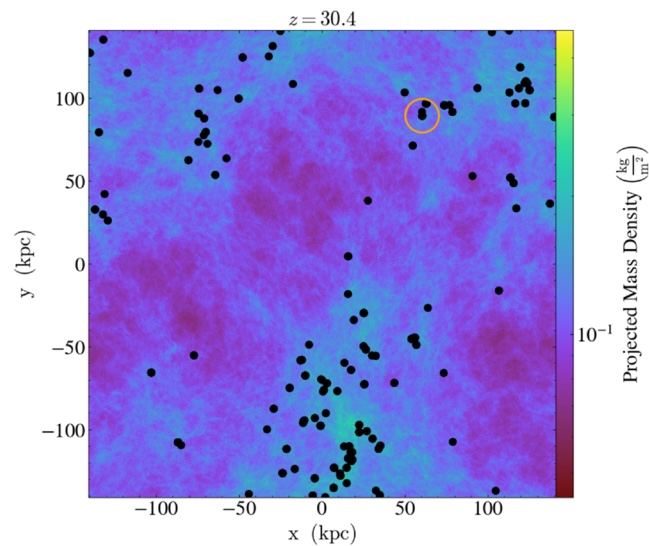
projection of the gas density in the simulated overdense region at z = 30.4

Figure 1: A projection of the gas density in the simulated overdense region at z = 30.4. The densest structures stand out clearly, tracing the locations where the first stars are able to form. Black dots mark newly formed groups of stars, while the most massive dark matter halo in the region is highlighted with an orange circle. The figure illustrates that in such an unusually dense patch of the early universe, star formation can already be underway just 100 million years after the Big Bang, creating the conditions needed for early Population III stars and their explosive deaths. [Adapted from Jeon et al. 2026]

In their simulations, star formation begins as early as z ~ 30–40 (within the first hundred million years after the Big Bang), producing Population III stars and, by extension, potential PISNe very shortly afterwards. While such overdense regions are rare, the authors show that the total area already surveyed by JWST (including large surveys such as CEERS, JADES, PRIMER, and COSMOS-Web) is large enough that it is plausible JWST has already observed at least one such region.

Catching a Cosmic Explosion in the Act

So, we can tick off condition #1: it’s possible that a sufficiently overdense region has already been observed by JWST. Next up, how lucky do we have to be to catch an explosion in the act (condition #2), so to speak? For this condition, cosmic time dilation actually works in our favour. A PISN explosion at z > 20 that lasts only months in its own rest frame can last for decades in the observed frame. (This whole time-being-relative thing sounds wacky because it is — please join me, Neil deGrasse Tyson, and countless others in struggling to imagine this.)

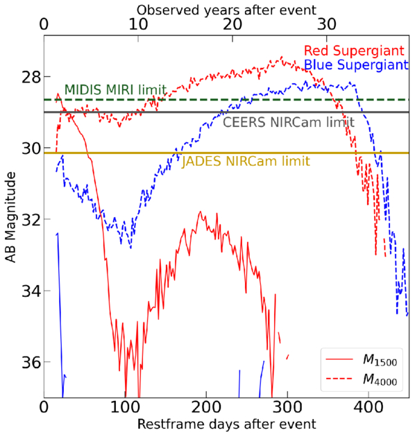
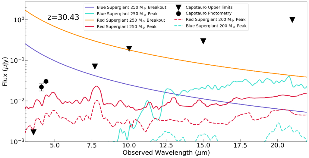
But would any such explosion be bright enough (condition #3)? Using theoretical PISN spectra, the authors show that these explosions could reach observed magnitudes of ~28–29 at z ~ 30 — right at the depth of current JWST deep surveys (Fig. 2). In fact, the predicted brightness and colours are somewhat comparable to those of some proposed z ~ 30 candidates (Fig. 3), raising the possibility that these objects could be PISNe rather than galaxies.
plot of predicted PISN brightness

Figure 2: This plot compares the predicted brightness of PISNe originating from different types of extremely massive stars to the depth reached by existing JWST surveys, showing that these explosions could remain detectable for ~20 years at peak brightness in the observed frame. [Jeon et al. 2026]
Theoretical PISNe spectra compared to a proposed z = 32 source

Figure 3: A comparison of theoretical PISNe spectra with the observed photometry of one proposed z ≈ 32 source (Capotauro). The coloured curves show model spectra for PISNe originating from extremely massive stars, at different stages of the explosion, while the data points represent the observed brightness of the high-redshift candidate across multiple JWST filters. [Jeon et al. 2026]

So… Are We Seeing the First Stars Die?

It’s not time to throw a party just yet. The authors note there are several caveats and uncertainties. The nature of Population III stars is still highly uncertain, JWST does not continuously monitor the same patch of sky, and identifying a PISN at such high redshift would be extremely challenging. Thanks to time dilation, these explosions would fade very slowly, making them hard to distinguish from steady sources using photometry alone. Alternatively, there are other plausible explanations for these ultra-high-redshift candidates: lower-redshift interlopers (a rather infamous example is CEERS-93316), local brown dwarfs, or even nearby exoplanets.

Still, the idea is exciting. If JWST were to detect a genuine PISN at z > 20, it would represent a direct glimpse of the very first stars, pushing observational astronomy into truly uncharted territory. For now, the most distant explosions in the universe may already be hiding in JWST images; we just have to learn how to recognise them.

Original astrobite edited by Nathalie Korhonen Cuestas.

About the author, Lucie Rowland:

I’m a fourth (and final!) year PhD student at Leiden Observatory in the Netherlands, studying massive, star forming galaxies in the early universe with ALMA and JWST. It’s a really exciting time to be interested in astronomy, so I hope to make groundbreaking new research more accessible!

The post The Oldest Starlight appeared first on AAS Nova.

  •  

How Galaxies Grow Up

JWST unfolded against a black background.

How do galaxies grow? A massive survey from JWST can help astronomers answer that fundamental question about galaxy evolution.

Time Machines

A photograph of thousands of galaxiesin one frame.

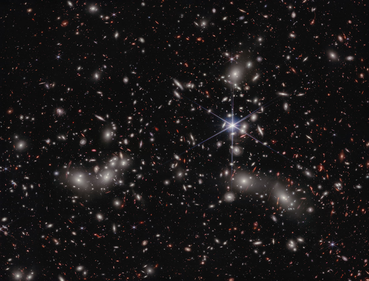
An image taken by JWST’s NIRCam instrument, the primary instrument behind the COSMOS-Web survey, of Pandora’s Cluster. Click to enlarge. [NASA, ESA, CSA, Ivo Labbe (Swinburne), Rachel Bezanson (University of Pittsburgh); Image Processing: Alyssa Pagan (STScI)]

When astronomers look into the night, they are greeted by a sky full to bursting with galaxies. But immediately after the Big Bang, none of these grand structures could have existed in our universe: all of the matter was too hot and dense to collapse into the whirlpools and ellipses we see today. We know that it took time for dark matter to collapse into halos, for gas to cool and fall into those halos, and even more time for those halos to merge together and galaxies to form. However, quantifying that story is tricky. How long did it take for the gas to cool and collapse? How often did small galaxies merge? How did the birth and death of stars play into all of this?

One way astronomers could go about answering these deep, fundamental questions in galaxy evolution would be to look at many galaxies spread across different distances. Famously, since the speed of light is fairly slow (cosmically speaking), we can only see distant objects as they appeared in the past. (This is why any aliens looking toward Earth from 65 million light-years away — from within the Virgo Cluster, perhaps — would see our planet as it was when dinosaurs roamed free.) In principle, then, by looking at a progression of galaxies farther and farther away, astronomers could convert these still images into a sort of movie of how typical galaxies look moving further and further back in time.

Seeing Red

There is a complication to this strategy, however. The farther away an object is, the more the light it emits is stretched towards redder wavelengths. As a consequence, any telescope designed to detect visible light won’t see anything; to take pictures of these galaxies, we need to build detectors that are specifically sensitive to stretched-out, near-infrared light.

This is one of the primary reasons that JWST was designed, constructed, and flung into space. It was purpose-built to collect and analyze near-infrared light from distant galaxies, and now after several years of observations and data crunching, astronomers are finally getting some answers to those fundamental questions.

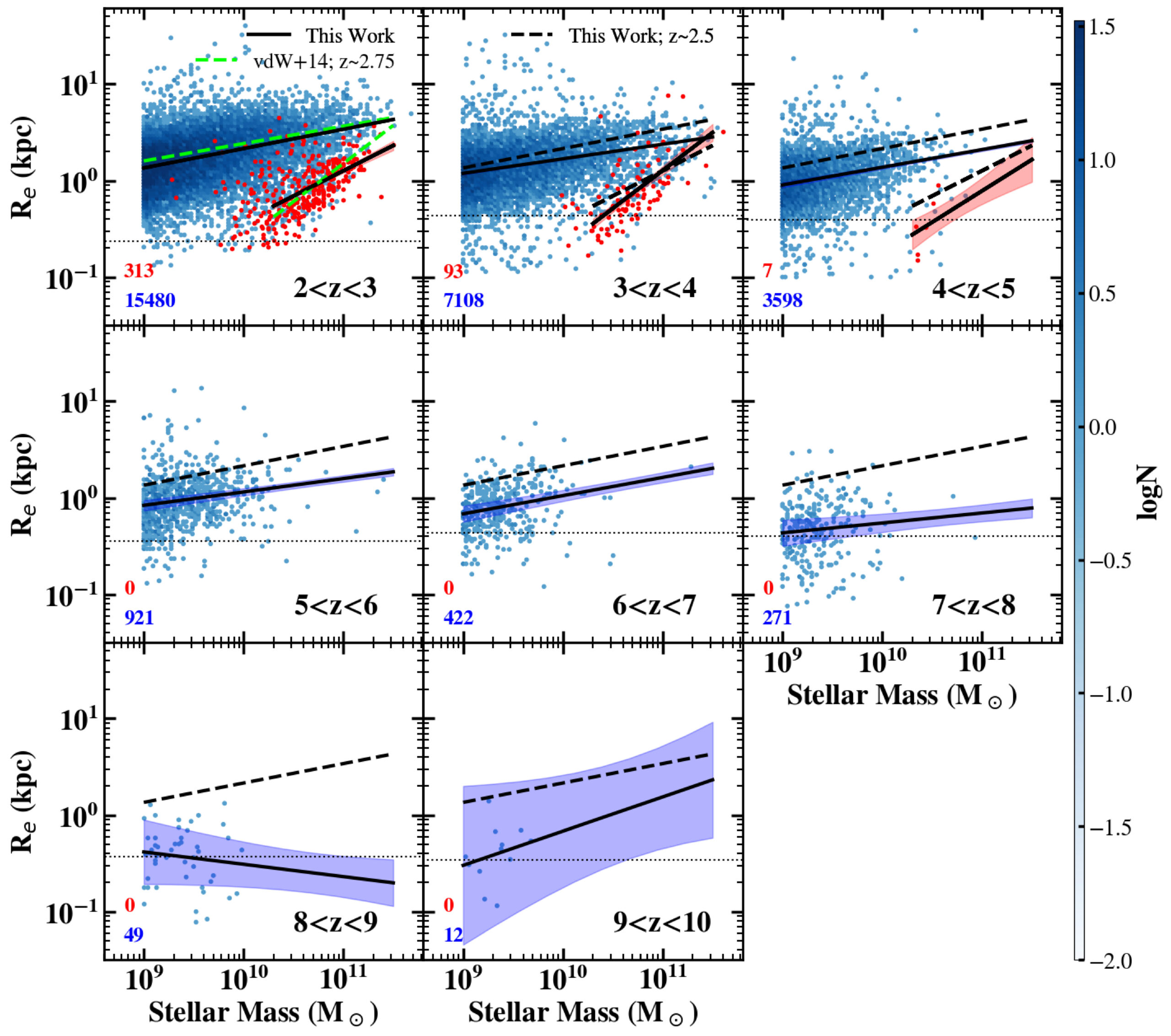
The results of how galaxies’ masses relate to their total size in different redshift bins. Click to enlarge. [Yang et al. 2025]

A Massive Survey

Recently, a team led by Lilan Yang, Rochester Institute of Technology, released their analysis of one of the earliest and largest surveys JWST has undertaken, a program called COSMOS-Web. The researchers mined a patch of sky about the size of the full Moon and extracted more than 30,000 distant galaxies, most of which had never before been seen by human eyes. They measured the brightness and size of each one and grouped them according to their redshift (a proxy for their distance) and whether they were actively forming stars or not.

The team found that, unsurprisingly, galaxies tend to grow over time. Excitingly, however, they also found that for star-forming galaxies, the relationship between a galaxy’s mass and its size is fairly constant for redshifts of z = 2–8. The scaling law between them also nicely matches up with measurements taken by the Hubble Space Telescope at smaller redshifts. Beyond that, though, for redshifts of z = 8–10, it’s possible that the scaling changes, though the authors emphasize that their sample is much smaller in these distant bins.

While more data are needed to confirm whether the youngest of these galaxies grow at a different pace than their later counterparts, we can be comforted that studies like this represent just our very first peek into a whole new era of galactic evolution, and that many more insights are sure to come as JWST keeps snapping images.

Editor’s Note: This article previously contained an error relating to the distance at which aliens would see Earth as it was when inhabited by dinosaurs. This error was corrected on 4 May 2026.

Citation

“COSMOS-Web: Unraveling the Evolution of Galaxy Size and Related Properties at 2 < z < 10,” Lilan Yang et al 2025 ApJS 281 68. doi:10.3847/1538-4365/ae0e1b

The post How Galaxies Grow Up appeared first on AAS Nova.

  •  

A Possible GLIMPSE of the Universe’s First Stars

Population III stars

Editor’s Note: Astrobites is a graduate-student-run organization that digests astrophysical literature for undergraduate students. As part of the partnership between the AAS and astrobites, we occasionally repost astrobites content here at AAS Nova. We hope you enjoy this post from astrobites; the original can be viewed at astrobites.org.

Title: GLIMPSE: An Ultrafaint ≃105 M⊙ Pop III Galaxy Candidate and First Constraints on the Pop III UV Luminosity Function at z ≃ 6–7
Authors: Seiji Fujimoto et al.
First Author’s Institution: University of Toronto; The University of Texas at Austin
Status: Published in ApJ

You, me, your laptop, my $8 matcha, and just about everything else on Earth was forged in the fiery bellies of dying stars. Generations of stars had to live and die before the universe became enriched with any elements heavier than helium (what astronomers call “metals”). The first stars to undergo this cosmic cycle are known as Population III (Pop III) stars. Though their existence has been hypothesized since the 1960s, astronomers have failed to observe these distant metal-free stars or the faint, low-mass galaxies that host them.

The first Pop III stars likely formed around 100 million years after the Big Bang in pristine pockets of hydrogen gas. Although these are too distant for us to observe, we expect that as the universe started to become metal enriched, there were still existing pockets of gas introverted enough to survive unpolluted and form metal-free Pop III stars up to a redshift of z ~ 6–7 (when the universe was around 900 million years old)!

JWST is the perfect instrument to search for these systems. You can read other astrobites on the search for possible Pop III systems with JWST here and here. The authors of today’s article seek to develop the most efficient way of using JWST’s Near-Infrared Camera (NIRCam) to find the galaxies hosting Pop III stars. Using their selection method on existing NIRCam data, the authors identified one promising Pop III galaxy candidate.

I’m Not Like Other Galaxies

In order to find a Pop III galaxy, we need to take a look at galaxies’ spectral energy distributions (SEDs). These are graphs that show the energy emitted by a galaxy at different wavelengths of light. Pop III galaxies are expected to have SEDs that differ from your everyday, metal-enriched galaxy. NIRCam will be especially sensitive to three key spectral features that show up in the SEDs of Pop III galaxies: an absent [O III] line (light emitted by doubly ionized oxygen atoms), a strong H-alpha line (light emitted when a hydrogen atom transitions from its third to its second energy level), and a significant Balmer jump (light absorbed to ionize electrons in the second energy level of a hydrogen atom). To identify these key SED characteristics, the authors use SED fitting and color–color diagrams to execute an efficient Pop III search with NIRCam.

The first selection method involves SED fitting. Astronomers create template SEDs that represent different types of galaxies and then compare these templates to the observed SEDs to see which one matches best. In this work, the authors use metal-rich galaxy templates and Pop III templates to fit the galaxies observed with NIRCam. They then calculate the chi-squared χ2 (a statistical measure of best fit) between the data and all the SED templates. A galaxy is selected as a Pop III candidate if the Pop III model provides a good fit (χ2 < 10) to the photometry and is significantly better than any metal-rich model. It’s kind of like looking for Cinderella by making every woman in the kingdom try on the glass slipper.

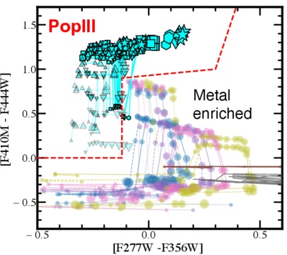
A color-color diagram showing how Pop III models lie in a different parameter space than metal-rich galaxies.

Figure 1: Color–color diagram for selecting Pop III galaxies where the x and y-axes show the different NIRCam filters being subtracted. The cyan symbols are different Pop III models while the other colored dots are different metal-rich galaxy models. [Adapted from Fujimoto et al. 2025]

A color–color diagram plots the difference in magnitude between two filters on each axis. NIRCam filters are specially chosen to emphasize the SED characteristics above. When these filters are chosen, Pop III galaxies occupy a distinct region of this diagram as compared to metal-rich galaxies. For example, subtracting the F356W filter from the F277W filter is sensitive to the presence of the [O III] line and the Balmer jump. Figure 1 demonstrates how this color selection separates Pop III galaxies from typical galaxies.

O Pop III, Pop III, Wherefore Art Thou?

The authors apply their fresh new selection criteria to publicly available NIRCam data from large surveys. And (drum roll please) the slipper fits! The Pop III galaxy candidate GLIMPSE-16043 is an ultra-faint galaxy at z = 6.5. It was imaged in the GLIMPSE survey, which uses the technique of gravitational lensing to observe faint and distant galaxies.

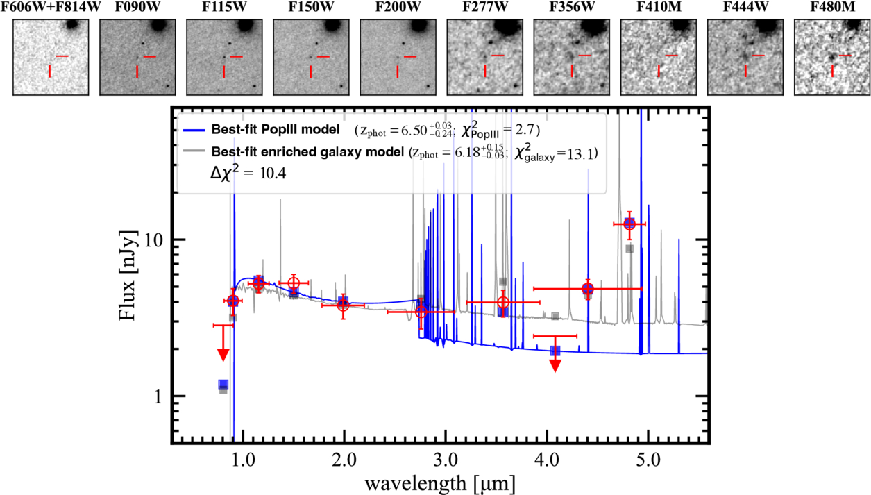
The GLIMPSE survey targeted a massive galaxy cluster, Abell S1063. The cluster bends the light from distant galaxies and, like a giant lens, magnifies faraway objects, providing some of the deepest JWST imaging to date. The Pop III candidate passes both tests: it resides in the Pop III region of the color–color diagram, and its SED is best fit by a Pop III model, not a metal-rich galaxy model (see Figure 2). Next, spectroscopic follow-up is needed to ensure that this galaxy is truly metal free and not just extremely metal poor.

The spectral energy distribution of a Pop III galaxy candidate. This plot shows that the JWST data is best fit by a Pop III model rather than a metal-rich galaxy.

Figure 2: SED of GLIMPSE-16043 with the best-fit Pop III template (blue) and best-fit metal-enriched template (gray). The top panel is the galaxy imaged in different filters from NIRCam and the Hubble Space Telescope. [Fujimoto et al. 2025]

The authors conclude that our best shot at identifying additional Pop III galaxy candidates is using NIRCam to image large numbers of gravitationally lensed clusters. Without magnification from gravitational lensing, it may be impossible to see these ultra-faint Pop III galaxies. Once candidates have been identified, they can be followed up with deep spectroscopy to confirm their redshift and their lack of metals. Who knows? With these new methods, we may soon get a glimpse of the universe’s very first stars.

Original astrobite edited by Chris Layden and Margaret Verrico.

About the author, Madison VanWyngarden:

I am a first-year PhD student in astronomy and NSF Graduate Research Fellow at the University of Arizona. I study galaxy formation and evolution in the distant universe and am particularly interested in dusty star-forming galaxies. In my free time, I love reading, hiking, and baking bread!

The post A Possible GLIMPSE of the Universe’s First Stars appeared first on AAS Nova.

  •  

Enhancing the Sharpest Images

The Submillimeter Array at the summit of Maunakea in Hawaiʻi.

The Event Horizon Telescope (EHT), the facility that delivered humanity’s first-ever picture of a black hole, can produce some of the sharpest images in all of astronomy. But turning the EHT’s raw data into images is a complex process involving messy statistics and powerful algorithms. Recent work presents a potential upgrade to that process: for the first time in long-baseline interferometry, it may be possible to model everything everywhere all at once.

The Hardest Eye Test

The EHT has some of the sharpest eyes in all of astronomy. With its effective resolution of just 20 microarcseconds, in principle you could use it to read a newspaper in New York while sitting at a cafe in Paris. But this planet-spanning instrument (it relies on data from radio telescopes on four continents) doesn’t snap pictures like an ordinary camera. Instead, each pair of telescopes measures something called an “interferometric visibility,” which is related to a single Fourier component of the actual underlying image.

A photograph of an orange ring surrounding a dark center.

The first image of a black hole, constructed from Event Horizon Telescope data taken in 2017. [EHT Collaboration; CC BY 4.0]

Combining these components into an image is a process fraught with assumptions and modeling choices. Since the EHT doesn’t have an infinite number of telescopes, each measurement can be mapped to infinitely many images. This forces researchers to choose how to “regularize” this space of images to select one best picture. Making things harder, they also must contend with all the typical issues of real-world data collection. Each telescope has slight calibration errors, and every data point is affected by weather and temperature-dependent processes.

Typically researchers break the problem down into several stages: first calibrate the data, then regularize and construct the best-fitting image, then analyze that image to constrain the actual physics you care about like the width of the ring surrounding a black hole. This is how the original EHT publications went about their groundbreaking work on the now-iconic glowing ring around the supermassive black hole in the galaxy Messier 87 (M87*).

A New Approach

Recent work led by Paul Tiede (Black Hole Initiative at Harvard University) suggests an alternative process. Instead of separating the stages of analysis as described above, the team demonstrated that one could fit everything simultaneously in a framework they call hierarchical interferometric Bayesian imaging, or HIBI.

A multi-panel plot of images of an orange blob with a tail. All images are very similar.

A comparison of the new HIBI technique (referred to as “Comrade” here) and a traditional algorithm called CLEAN. Click to enlarge. [Tiede et al. 2026]

By fitting all parameters that go into an image together, the method doesn’t select one “best” image. Instead, by allowing the pixel-by-pixel intensities, calibration parameters, and underlying physics to inform one another during inference, HIBI explores the full range of images consistent with the data. This prevents the degeneracies that plague the traditional approach, where image and calibration estimates can trade off against each other in misleading ways. The team validated HIBI on synthetic data mimicking the EHT’s 2017 setup, showing that it reliably recovered a range of source shapes with well-calibrated uncertainty estimates.

Even more exciting, the team demonstrated that it’s possible to skip the image construction step altogether and go straight to the science. By fitting parameters describing the physics underlying a scene, the team was able to constrain the width of the ring around M87* without any reference to a picture. They predict that this technique could be crucial for extracting information when future instruments like the Next Generation Event Horizon Telescope observe more distant black holes that are only marginally resolved. Though we’ll likely have to wait years for these next-generation telescopes, work like this ensures that astronomers will be able to squeeze as much science from them as possible once these new facilities are ready.

Citation

“Hierarchical Interferometric Bayesian Imaging,” Paul Tiede et al 2026 ApJ 997 262. doi:10.3847/1538-4357/ae2749

The post Enhancing the Sharpest Images appeared first on AAS Nova.

  •  

Observing the End of Star Formation in Galaxies

galaxy transitioning from star forming to quiescent

Editor’s Note: Astrobites is a graduate-student-run organization that digests astrophysical literature for undergraduate students. As part of the partnership between the AAS and astrobites, we occasionally repost astrobites content here at AAS Nova. We hope you enjoy this post from astrobites; the original can be viewed at astrobites.org.

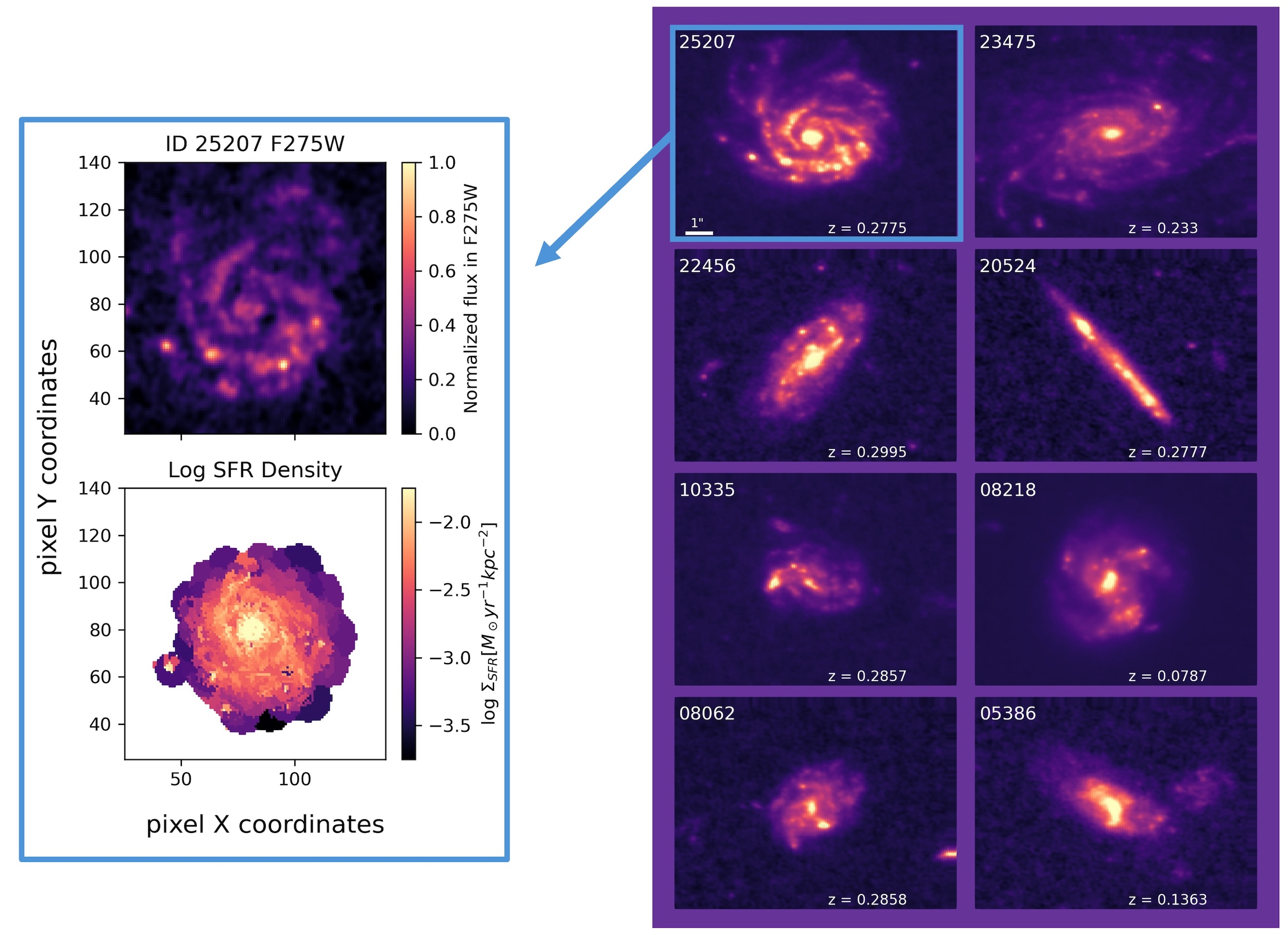
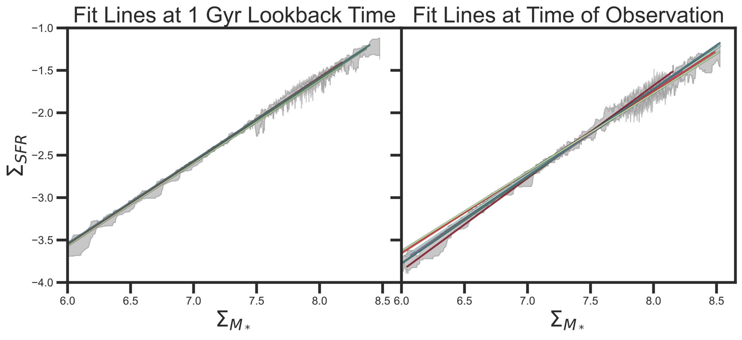
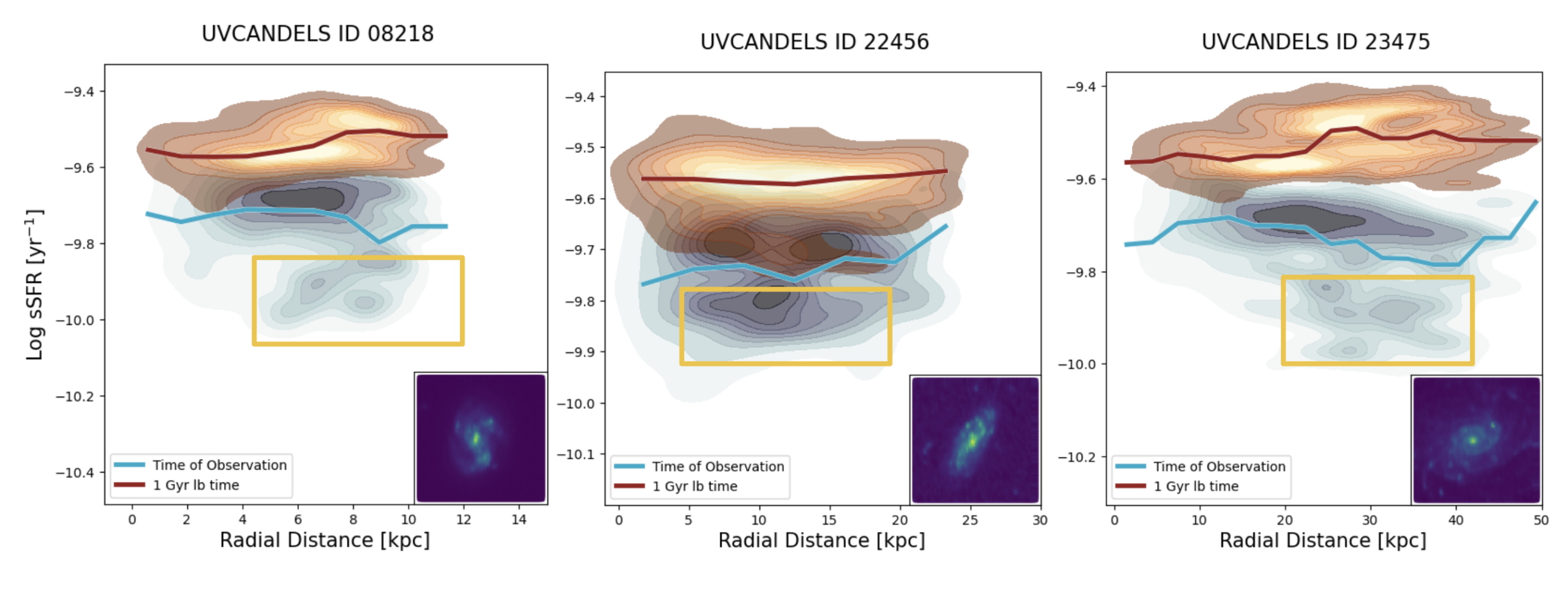
Title: Searching Within Galaxies for the Earliest Signs of Quenching With Spatially Resolved Star Formation Histories in UVCANDELS
Authors: Charlotte Olsen et al.
First Author’s Institution: New York City College of Technology
Status: Published in ApJ

How and Why Do Galaxies Stop Forming Stars?

Galaxies serve as important laboratories for many subfields of astrophysics. As such, astrophysicists are interested in the full galactic life cycle, from how galaxies are born to the end of their formation. Whereas young galaxies in the distant universe are actively forming stars, many nearby galaxies are much quieter, with little or no ongoing star formation. Astronomers like to describe these galaxies as “red and dead” because their stars are older and therefore appear redder in color. The process by which galaxies shut down their star formation is known as quenching, and it causes galaxies to become quiescent. Understanding the origin of quiescent galaxies is a fundamental question in galaxy evolution. Studying this process is challenging, however, because star formation is intertwined with many other factors that shape galaxies, including their environments and supermassive black holes.
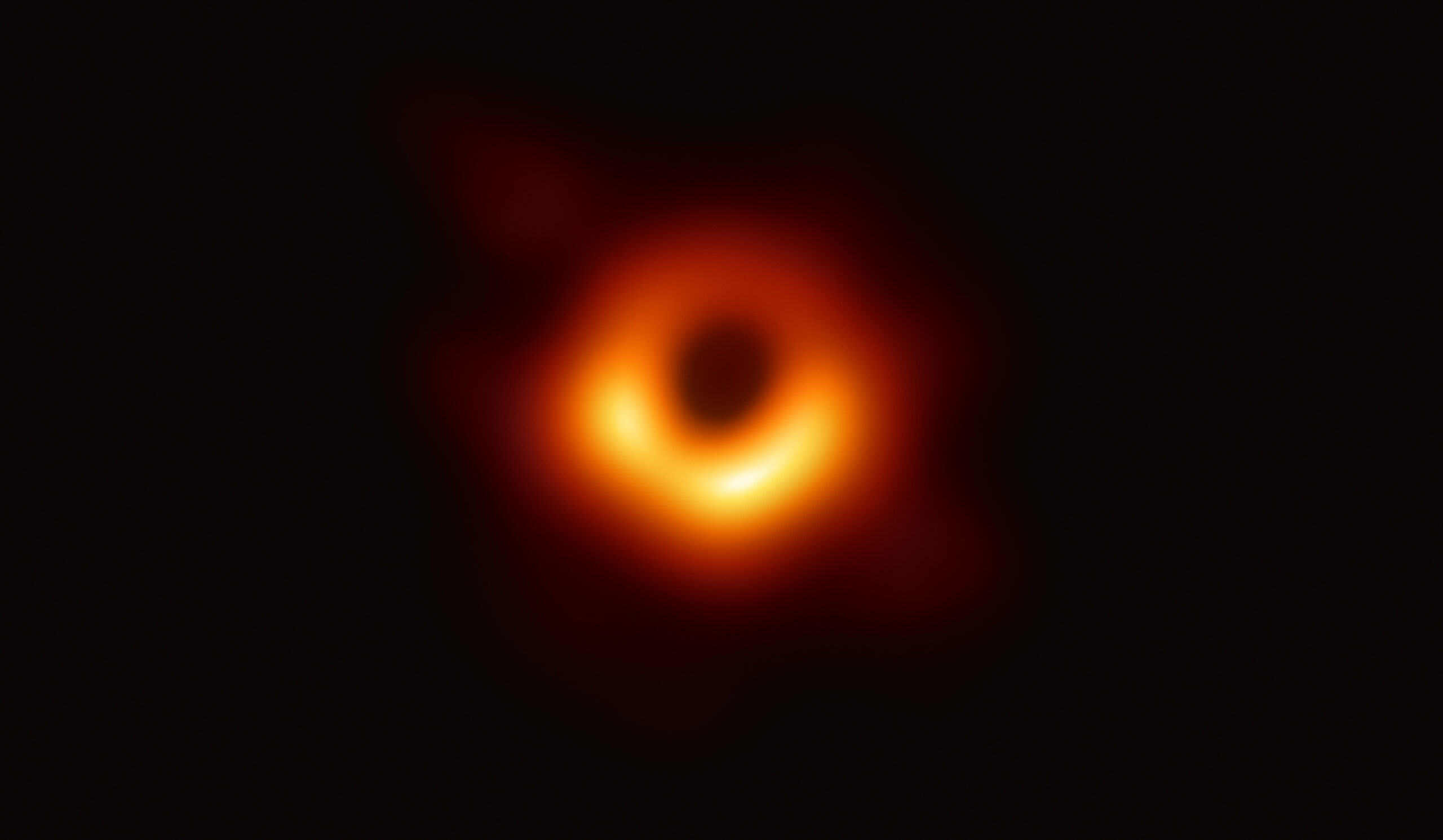
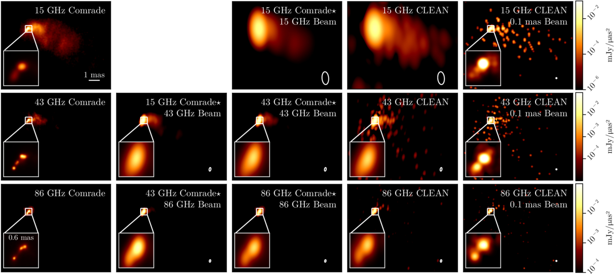
Star formation occurs on scales that are much smaller and over timescales much shorter than the global properties and overall lifetime of a galaxy. By observing star formation on these smaller scales over time, astronomers can gain a clearer picture of how star formation ceases in a galaxy, and they can determine whether this process is driven from the inside out — starting with the supermassive black hole in the galactic center — or from the outside in, influenced by environmental effects. In today’s article, the authors use the Cosmic Assembly Near-Infrared Deep Extragalactic Legacy Survey with high-resolution ultraviolet coverage (UVCANDELS) to examine eight “golden” galaxies, shown in Figure 1. They then reconstruct the star formation histories within small regions of each galaxy to detect the “earliest signs of quenching.”

galaxy sample from Olsen et al.

Figure 1: Images of the eight galaxies in the “Golden Sample” of galaxies studied in this work (right). These galaxies were chosen because of their clear detection, and they show a range of edge-on to face-on views as well as shapes. The authors divided each galaxy into small, resolved regions in which they measured the star formation (example shown on left). [Adapted from Olsen et al. 2026]

Characterizing the Star Formation Histories

To trace a galaxy’s star formation over cosmic time, today’s authors model its integrated light — which encodes the many episodes of past star formation — using spectral energy distribution (SED) fitting. By comparing a galaxy’s light across many wavelengths to computer models, SED fitting can estimate the ages of its stars and when they formed. This approach allows astronomers to study how a galaxy’s star formation rate evolves as a function of its stellar mass, known as the SFR – Mstellar relation. Note that the article considers the star formation rate and stellar mass in individual regions of each galaxy, so it analyzes these properties as surface densities, ΣSFR and ΣMstellar, instead of the total values.

Using SED fitting, the authors determine the expected star formation rate and stellar mass of the regions from 250 million to 1 billion years before the time of observation. Figure 2 shows the line of best fit for the SFR – Mstellar relation of the regions for each galaxy, before and at the time of observation. The SFR – Mstellar relations are very similar across the sample 1 billion years before the observations; however, by the time of observation, the overall star formation rates have decreased slightly, indicating that the galaxies are beginning to quench. They also exhibit increased variation suggesting that each galaxy is quenching in a different way.

best-fit SFR – M stellar relation

Figure 2: The best-fit SFR – Mstellar relation of the regions for each galaxy, represented by the different colored lines, 1 billion years (1 Gyr) before and at the time of observation (left and right panels, respectively). At 1 billion years before the observation, the galaxies appear to have the same relation, but their variation at the time of observation suggests that the galaxies have begun quenching in different ways. [Olsen et al. 2026]

To further probe how these galaxies are starting to quench, the authors also measure the specific star formation rate (sSFR) of the regions as a function of their distance from the center of the galaxy. The sSFR can be thought of as the rate of new star formation relative to the amount of existing stellar mass: SFR /Mstellar. Figure 3 shows three examples from the galaxies studied in this work. Once again, the star formation rates of the regions decrease over the course of 1 billion years. However, the regions where the star formation rate has declined most rapidly differ from galaxy to galaxy — ranging from the central regions to the mid-disk to the outskirts — as each galaxy is undergoing a different quenching mechanism.
specific star formation rate of the regions as a function of their distance from the center of the galaxy

Figure 3: The specific star formation rate of the regions as a function of their distance from the center for three of the galaxies in the sample. Overall, the star formation rate decreases from 1 billion years before the observation (red) to the time of observation (blue). However, the regions where the star formation decreases most significantly (indicated with the yellow boxes) vary from galaxy to galaxy. [Olsen et al. 2026]

Detecting the Earliest Signs of Quenching

It should be noted that all of the galaxies in this study are still forming stars. However, they are on the verge of having their star formation suppressed, offering valuable insight into how quenching begins and how diverse the process can be. New telescopes are pushing the boundaries of what we can observe. On one hand, JWST can capture galaxies at exceptionally high resolution; on the other, the Vera C. Rubin Observatory and the Nancy Grace Roman Space Telescope will deliver vast datasets containing billions of galaxies. Future investigations leveraging these facilities could reveal more about the physical processes that quench galaxies on small scales, shedding light on the mechanisms that drive galaxy evolution.

Original astrobite edited by Catherine Slaughter.

About the author, Shalini Kurinchi-Vendhan:

After studying astrophysics and literature at Caltech, I moved onto a Fulbright Fellowship in Heidelberg, Germany. I’m passionate about using computer simulations to explore supermassive black holes and galaxy evolution — but I also love poetry and traveling.

The post Observing the End of Star Formation in Galaxies appeared first on AAS Nova.

  •  

A Potential New Piece of the “Little Red Dot” Puzzle

X-ray dot

Editor’s Note: Astrobites is a graduate-student-run organization that digests astrophysical literature for undergraduate students. As part of the partnership between the AAS and astrobites, we occasionally repost astrobites content here at AAS Nova. We hope you enjoy this post from astrobites; the original can be viewed at astrobites.org.

Title: The X-Ray Dot: Exotic Dust or a Late-Stage Little Red Dot?
Authors: Raphael E. Hviding et al.
First Author’s Institution: Max Planck Institute for Astronomy
Status: Published in ApJL

What Are Little Red Dots?

One of the most intriguing results produced by JWST was the serendipitous discovery of a new class of object: “little red dots” (LRDs). These objects started popping up everywhere in our early universe observations. Surprisingly, they look like compact (little) red dots in imaging data (astronomers are an incredibly creative bunch). The number of LRDs we observe drops drastically at redshifts less than about z = 4 (about 12 billion years ago), implying that LRDs are likely evolving into something else entirely. The luminous, compact nature of LRDs, paired with their disappearance from the cosmic stage, has continuously puzzled astronomers in recent years.

At least part of the LRD population has routinely been explained as a new class of active galactic nuclei (AGN). AGN are the central engines of many galaxies — luminous regions powered by actively accreting supermassive black holes. Recent evidence has increasingly pointed towards LRDs being a new class of AGN: black hole stars, or black holes surrounded by dense cocoons of gas. Naturally, this raises questions surrounding the placement of LRDs in our understanding of supermassive black hole and galaxy evolution across cosmic time.

A hallmark of typical AGNs is their X-ray brightness. X-rays are one of the most energetic types of electromagnetic radiation, and they are primarily produced by the most extreme astrophysical situations (think neutron star mergers). One of the key challenges in explaining the nature of LRDs has been their lack of X-ray emission. Their lack of emission in this regime is a piece of evidence pointing towards a black hole star scenario — dense gas can block the X-rays being produced by the black hole. However, the lack of LRDs in the present-day universe implies that they likely shed their cocoons at some point. Catching an LRD in the act of shedding its cocoon would thus provide an important piece of evidence surrounding their nature and evolution. Thankfully, today’s authors may have done exactly that! They report the discovery of what they call the “X-ray dot” (XRD): an LRD-like object that is also X-ray luminous at a redshift of approximately z = 3.28.

New JWST Observations of the XRD

While archival observations of the XRD with the Hubble Space Telescope, the Canada France Hawaii Telescope, the Spitzer Space Telescope, and the Chandra X-ray Observatory existed, new spectral data from JWST were needed to study the system in depth. Spectral data have a huge advantage over photometric observations when it comes to modeling the system. With a good quality spectrum, astronomers can use sophisticated modeling tools to try and pin down the physical nature of the emission we’re observing, and thus understand its intrinsic nature.

Figure 1 showcases the archival data from Hubble, Spitzer, and Chandra, along with the XRD’s spectrum from JWST (black curve, bottom panel). Photometric observations of the source indicate that it is incredibly compact (radius ≲ 250 pc, about 100 times more compact than the Milky Way) and shows similarities to LRD spectra, but with some key differences. (An example LRD spectrum is shown as the red curve in Figure 1.) The impressive X-ray luminosity of the XRD — typical of standard AGNs — is another key difference between it and standard LRDs.

A figure showing image cutouts from HST, Spitzer, and Chandra, of the XRD. The bottom panels also shows its spectrum alongside a typical LRD spectrum.

Figure 1: Top: Image cutouts from various Hubble, Spitzer, and Chandra observations of the XRD. Bottom: The spectrum of the XRD (black) shown alongside a similar LRD spectrum (red) and two quasar spectra (blue and purple), one of which has been reddened due to the presence of dust (purple). [Hviding et al. 2026]

So…What’s the Deal with the XRD?

To understand the nature of the XRD, the authors fit a variety of models describing a wide range of physical systems to the available data. Surprisingly, their best-fit models indicate that if the XRD is simply a typical AGN heavily obscured by astrophysical dust, its dust properties are drastically different from those of typical galaxies and AGN. Instead, trying to explain the system as an AGN embedded in a cocoon of gas (the black hole star model) provides better results (more aligned with observed LRDs), but it still isn’t perfect.

Notably, the emission in the ultraviolet-to-optical regime of the electromagnetic spectrum differs greatly from that of LRDs. In LRDs, this emission is indicative of a single dense gas component around the supermassive black hole, while in the XRD the authors find evidence suggestive of a patchier, less uniform distribution of gas. However, in order for this explanation to match the data, physical conditions of the model must be finely tuned, suggesting that this model may need to be refined further. These factors seem to suggest that the XRD is poorly understood in the context of our current paradigm of models describing AGNs and LRDs. The potentially patchy nature of the XRD’s gas envelope could suggest that this object is an LRD in the process of shedding its outer envelope, evolving into a typical AGN.

Regardless of its true nature, the XRD opens up new doors in our understanding of AGNs and LRDs. It provides an exciting glimpse at AGN evolution in action — a transitional fossil for early universe black holes. With a new piece of the puzzle slotted into our picture of AGN evolution, it’s only a matter of time before astronomers fully contextualize the stubbornly enigmatic LRDs.

Original astrobite edited by Ansh R. Gupta.

About the author, Drew Lapeer:

Drew is a first-year PhD student at the University of Massachusetts Amherst. They are broadly interested in the evolution of galaxies, with a focus on the impact of cosmic feedback on the galactic ecosystem. In their free time, they enjoy reading, rock climbing, hiking, and baking!

The post A Potential New Piece of the “Little Red Dot” Puzzle appeared first on AAS Nova.

  •  

Detecting New Icy Molecules Around a Newly Forming Star with JWST

Large Magellanic Cloud

Editor’s Note: Astrobites is a graduate-student-run organization that digests astrophysical literature for undergraduate students. As part of the partnership between the AAS and astrobites, we occasionally repost astrobites content here at AAS Nova. We hope you enjoy this post from astrobites; the original can be viewed at astrobites.org.

Title: Protostars at Subsolar Metallicity: First Detection of Large Solid-State Complex Organic Molecules in the Large Magellanic Cloud
Authors: Marta Sewiło et al.
First Author’s Institution: NASA Goddard Space Flight Center
Status: Published in ApJL

Stars and planets form when clouds of molecules collapse in on themselves due to the overwhelming force of gravity (which, relatable). This process is quite mysterious, as these clouds will only live for a couple million years before collapsing, and the newly forming protostars only live for about half a million years before becoming main-sequence stars.

But we are able to find some protostars in the Milky Way and in the Small and Large Magellanic Clouds near us, and observing the molecules around these protostars can help us understand how protostars form.

To look for molecules around protostars, astronomers take spectra of the protostars in the infrared, which is a wavelength region where molecules emit a lot of light. As better instruments are being built, astronomers are more often able to look for what are called complex organic molecules, which are carbon-bearing molecules with at least six atoms.

These complex organic molecules can be detected in different states: most detections have been of gaseous molecules in and around protostars or planet-forming disks, but they can also be found in a solid state on the surfaces of dust grains in the interstellar medium in a galaxy. In this state, they are called complex organic molecule “ices.” These “ices” were rarely found pre-JWST, but since its launch, detections have been more numerous, mainly in the Milky Way. Observing these complex molecules on the surfaces of dust grains tells us more about protostellar dust chemistry, which is an important but still mysterious aspect of star formation.

In this study, researchers look outside of our own galaxy to explore the complex organic molecules in the Large Magellanic Cloud (LMC). The LMC is an interesting place to look for these molecules because it has lower metal content (i.e., elements heavier than hydrogen and helium) than the Milky Way, as well as a harder radiation field. This means photons flying around in the LMC generally have higher energies than photons flying around in the Milky Way, and elements like carbon, oxygen, and nitrogen are less abundant. This is important because these conditions are more similar to what typical galaxies were like in the early universe. Thus the LMC is a better test bed to look at protostars than the Milky Way if we want to understand how stars formed in the early universe.

The authors of this study have found signatures of complex organic molecules in protostars forming in the LMC. They focus on the protostar ST6 in the LMC, shown in the right image in Figure 1. They used JWST’s Mid-Infrared Instrument to take spectra of the region around ST6.

Large Magellanic Cloud and N158

Figure 1: The LMC (left) and a zoomed-in view of region N158 (right) containing protostar ST6, the focus of this study. In the inset panel of the right picture, contours of carbon monoxide emission are shown. [Sewiło et al. 2025]

Spectroscopic Signatures of Molecules on Dust Grains

The researchers used the Python tool called dEcompositioN of Infrared Ice features using Genetic Modelling Algorithms (ENIIGMA) to fit the spectroscopy. This code compares the spectra to laboratory data of these complex organic molecules at the temperatures we see in the LMC. The authors fit for complex organic molecules they might expect to see, and they detect methanol (CH3OH), acetaldehyde (CH3CHO), ethanol (CH3CH2OH), methyl formate (HCOOCH3), and acetic acid (CH3COOH); of these, acetaldehyde, ethanol, and methyl formate have never before been detected outside of the Milky Way. Interestingly, this is the first time acetic acid has been definitively detected in any astrophysical environment. The spectral contribution from each molecule is shown in Figure 2; all the individual contributions added together make up the observed spectrum.

spectrum of the protostar ST6

Figure 2: Model fits to the spectrum of the protostar ST6 using the code ENIIGMA. Molecules and their fitted emission are given in the legend. [Sewiło et al. 2025]

These detections provide evidence that these complex organic molecules can be produced on the surfaces of dust grains. Further, their detection in the LMC provides evidence that these molecules can be produced in “harsh” environments like the LMC, with lower metal content and harder radiation fields.

When the authors compared the abundances of these ices to other protostars in the Milky Way galaxy, they found that the abundances are slightly lower around the LMC protostar. This may happen because the dust temperatures are generally higher in the LMC due to the higher-energy photons, which affect the chemistry happening on the dust. Some species they found, however, do have similar abundances to the Milky Way protostars, indicating that the harder radiation field of the LMC does not affect how these species form. Finding more complex organic molecules in the Magellanic Clouds will help us understand further how these compounds form on dust grains and how the galactic environment may affect their formation.

Original astrobite edited by Shalini Kurinchi-Vendhan.

About the author, Caroline von Raesfeld:

I’m a third-year PhD student at Northwestern University. My research explores how we can better understand high-redshift galaxy spectra using observations and modeling. In my free time, I love to read, write, and learn about history.

The post Detecting New Icy Molecules Around a Newly Forming Star with JWST appeared first on AAS Nova.

  •  

An Impostor Explosion

A rendering of two purple jets streaming away from a central explosion.

Over many centuries of observing the night sky, astronomers have found only a single visible afterglow of a collision between neutron stars. For a few days in the summer of 2025, it seemed like observers may have found another of these treasured but elusive prizes; unfortunately, the promising candidate turned out to be a supernova in disguise.

A Rare Prize

kilonova as seen by Hubble

These images from the Hubble Space Telescope show the fading light of the kilonova associated with the gravitational wave event GW170817. [NASA and ESA Acknowledgment: A. Levan (U. Warwick), N. Tanvir (U. Leicester), and A. Fruchter and O. Fox (STScI)]

When two neutron stars (the ultra-dense remnants of massive stellar explosions) spiral together and collide, the cataclysm is energetic enough to release strong gravitational waves, forge heavy elements, and briefly glow across the electromagnetic spectrum. These events are called kilonovae, and they’re quite rare; while we may have detected a handful at high energies, there is only one event for which astronomers managed to record both gravitational waves and an optical transient.

That one kilonova, found back in 2017, taught astronomers much about how heavy elements are formed and left the scientific community hungry for more data. Since then, each time a gravitational wave detector like LIGO reports that it may have spotted a neutron star merger, telescopes across the world scramble to look in the probable region of the sky, hoping to find the short-lived electromagnetic counterpart.

Too Good to Be True

On 18 August 2025, the LIGO/Virgo/KAGRA collaboration sent out an alert that it may have detected a neutron star–neutron star merger. The odds that their signal was real weren’t great, and the researchers gave it just a 29% chance of being a genuine astrophysical signal. Still, given the potential payoff of finding the next kilonova, several telescopes quickly began searches for the optical counterpart. The gravitational wave signal suggested that the event likely came from a curved patch of sky delightfully referred to as the “northern banana,” and after trawling that region for a few nights, astronomers hauled in 47 new transients. Any one of these could have been the kilonova, and all of them received extensive follow-up observations.

A team led by James Gillanders (University of Oxford) recently summarized some of these follow-up observations carried out with the Pan-STARRS and ATLAS telescopes. In the initial exciting few days after the alert went out, one candidate transient stood out as the most promising. Named AT2025ulz, it was first spotted by the Zwicky Transient Facility and initially started fading rapidly and changing colors, just as models of kilonovae predict. For four days, it seemed like the world may have witnessed its second-ever kilonova. But then the telescopes began their fifth night of observations.

Supernova Unmasked

A scatter plot showing a rapidly fading, then reversing and spiking, light curve.

The light curve of SN2025ulz. Note that the source appeared to grow brighter again after about 5 days. Click to enlarge. [Gillanders et al. 2025]

The light curve of AT2025ulz, after fading steadily in the preceding days, suddenly turned upwards; in other words, whatever was causing the transient got brighter. Models of kilonova evolution predict no such brightening, but Type IIb supernovae are known to follow just this behavior. AT2025ulz showed itself to be another run-of-the-mill stellar explosion, not the sought-after fireworks of two neutron stars slamming together.

Frustrating as this particular result may be, the effort was far from wasted. The team could use their non-detection of the true kilonova to place limits on its timing and peak magnitude, assuming it existed in the first place. And, as gravitational wave detectors grow more sensitive and alerts like this more common, hindsight will likely frame this scramble as a dress rehearsal for an ultimately successful kilonova recovery effort. Until then, astronomers will keep searching, and will keep their guard up against cosmic impostors.

Citation

“Pan-STARRS Follow-Up of the Gravitational-Wave Event S250818k and the Light Curve of SN2025ulz,” J. H. Gillanders et al 2025 ApJL 995 L27. doi:10.3847/2041-8213/ae2125

The post An Impostor Explosion appeared first on AAS Nova.

  •  

Triple Double: Do Merging White Dwarfs Produce Fast Radio Burst–Emitting Remnants?

Illustration of two white dwarfs about to merge

Editor’s Note: Astrobites is a graduate-student-run organization that digests astrophysical literature for undergraduate students. As part of the partnership between the AAS and astrobites, we occasionally repost astrobites content here at AAS Nova. We hope you enjoy this post from astrobites; the original can be viewed at astrobites.org.

Title: Fast Radio Bursts from White Dwarf Binary Mergers: Isolated and Triple-Induced Channels
Authors: Cheyanne Shariat et al.
First Author’s Institution: California Institute of Technology
Status: Published in ApJL

The History of Fast Radio Bursts

Since the discovery of the Lorimer Burst in 2007, astronomers have studied fast radio bursts (FRBs) in extreme detail. However, these extragalactic millisecond-duration radio transients have remained an enigma. Like many astrophysical phenomena, their discovery was serendipitous. The most prolific FRB-discovery instrument, CHIME, was not originally built to study them; the acronym stands for “Canadian Hydrogen Intensity Mapping Experiment,” reflecting its original (and ongoing) mission to map the cosmological distribution of hydrogen in the primordial universe. Since its construction, CHIME has discovered several thousand FRBs and even identified a smaller fraction that are known to repeat, some with consistent periods and others that are sporadic and seemingly random. (Check out their live catalog of repeating sources.)

Despite having thousands of sources to study, the only thing we know fairly confidently about FRBs is that many of them are extragalactic, and some others are even at cosmological distances. If we don’t understand how FRBs are produced, how can we know their distance? FRBs display a unique signature in their radio spectra, where higher frequencies arrive at the telescope first and lower frequencies arrive later, delayed by an inverse frequency-squared relationship. In a “dynamic spectrum,” this makes the pulse actually appear like a sweep from high to low frequency that follows the shape of a parabola; for example, the brightest pixels in Figure 1 of this Bite display this sweeping shape. This effect results from the FRB propagating through an ionized plasma with a specific density. Since the FRB is ultimately an electromagnetic wave, this slows down the speed of the FRB as a function of frequency. Measuring this effect, called dispersion, allows us to infer that the FRB signal passed through more plasma than can be accounted for within our own Milky Way galaxy, indicating that the FRB must have originated from much farther away. So far, there is only one example of an FRB from within our own galaxy, which was identified as originating from a magnetar, a highly magnetic pulsar.

FRB Progenitor Candidates

Although we know that most FRBs are located at extragalactic or even cosmological distances, it’s still not clear what objects that can generate them. Since magnetars and other compact objects are often considered reliable progenitors of FRBs, understanding their populations and comparing them with observed FRBs may reveal the origin of FRBs. Candidate FRB progenitor systems are usually divided into “prompt” channels — like the collapse of a star into a magnetar during a core-collapse supernova — and “delayed” channels where the FRB engine is formed on longer timescales, like accretion-induced collapse of white dwarfs or compact-object mergers. Figure 1 displays several of these channels, particularly those considered in today’s article, in which stellar evolution results in the transfer of material from one star to another (accretion-induced collapse) or gravitational radiation allows two objects to inspiral and merge. These events could create highly magnetized white dwarfs or magnetars that may produce FRBs.

different pathways and their associated fractions for producing an FRB candidate

Figure 1: Three different pathways and their associated fractions for producing an FRB candidate. Depending on the mass and composition of the merging objects, an FRB candidate may be produced instead of causing the white dwarf to explode in a Type Ia supernova. These are the systems of interest in today’s article. [Shariat et al. 2026]

Simulating Hierarchical Triples

In today’s article, we’re considering the role of hierarchical triple star systems in producing FRB-emitting objects. A hierarchical triple consists of an inner binary and a distant, tertiary star; see the first panel of Figure 1. These systems may play an important role because many stars that become white dwarfs of at least 0.8 solar mass exist in hierarchical triples: 35% of 2-solar-mass stars and 50% of 8-solar-mass stars are in triples. Stars of both masses will end their lives as white dwarfs.

The tertiary star plays an essential role in increasing the likelihood of the inner binary interacting: the eccentric Kozai–Lidov (EKL) mechanism causes the inner orbit to oscillate between highly inclined (with respect to the orbit of the tertiary star) and highly eccentric. Unlike isolated binaries that aren’t excited in this way, the eccentric orbit phase causes the inner stars to pass much closer to each other, increasing the likelihood of interaction or even a merger that could produce an FRB-emitting remnant.

The authors of today’s article produced a realistic population of triple systems by sampling from empirically measured distributions of masses, periods, and orbital eccentricities. These distributions were derived from observations collected by the Gaia satellite, an all-sky optical telescope that has now observed more than one billion stars in the Milky Way. The authors also created a “control” sample of isolated binaries by removing the tertiary star from the same sample of systems. The systems were then evolved for an age randomly selected between 0 and 12.5 billion years to simulate “constant” star formation similar to that in the Milky Way. Finally, they reapply these simulations at three different “metallicities” — the fraction of elements other than hydrogen or helium relative to that of the Sun.

Figure 2 displays these two populations: the isolated binaries are shown as filled histograms, and the hierarchical triples are shown as histograms with dashed lines. Each column represents the three different progenitor classes considered in Figure 1. At solar metallicity, the delays to merging are greater in triples than in secular binaries, leading to more mergers overall (top left panel). At lower metallicities, there are fewer mergers in all progenitor pathways in triples than in isolated binaries due to changes in stellar evolution attributed to weaker winds and larger pre-white dwarf masses.

mergers as a function of time for different metallicities and formation pathways

Figure 2: The number of mergers as a function of time from the hierarchical triple’s formation, given different three metallicities (rows) and the three primary formation pathways for FRB-emitting merged remnants considered in Figure 1. Filled histograms are isolated binaries, dashed histograms are triples. [Shariat et al. 2026]

A Cosmic Population of FRBs

Since we can’t realistically track individual star systems from their formation to the end, we need to convert the delay-time distributions shown in Figure 2 to an observable. To do this, the authors combine the results of their simulations with measurements of the cosmic star formation rate — how many stars form per unit time as a function of the universe’s age — and the evolution of the universe’s metallicity as stars fuse hydrogen into heavier elements and return this material to the interstellar medium as these stars end their lives in shedding red giants or supernovae. This analysis produces the number of FRBs that should be observed as a function of distance or lookback time into the universe’s history, which is displayed in Figure 3.

number of FRBs expected as a function of cosmological redshift

Figure 3: The number of FRBs expected as a function of cosmological redshift. The present is to the left, the distant and early universe is on the right. The top panel shows the three formation channels, with binary and triple systems separated. The bottom panel displays the composite rate and compares it with empirical estimates from existing FRB observations. [Shariat et al. 2026]

This analysis reveals key measurable differences between lone binaries and hierarchical triples: most notably, binary white dwarf mergers peak later in the universe (redshift of z ~ 1), while single binaries peak earlier (redshift of z ~ 2). These results highlight the importance of including triples in FRB progenitors because they are more likely to contribute to populations at later times — making them closer and more easily detectable — in the total population of FRBs. Future instruments like CHIME with the new outriggers and the Deep Synoptic Array will expand the sample of FRBs to reach farther cosmological distances, with better localizations, enabling more statistically motivated tests of different formation pathways.

Original astrobite edited by Catherine Slaughter.

About the author, Will Golay:

I am a graduate student in the Department of Astronomy at Harvard University and the Center for Astrophysics | Harvard & Smithsonian, advised by Edo Berger. I study radio emission from transient astrophysical objects like tidal disruption events.

The post Triple Double: Do Merging White Dwarfs Produce Fast Radio Burst–Emitting Remnants? appeared first on AAS Nova.

  •  

I Survived a Type Ia Supernova, and All I Got Was This Kick Velocity

G272.2-3.2

Editor’s Note: Astrobites is a graduate-student-run organization that digests astrophysical literature for undergraduate students. As part of the partnership between the AAS and astrobites, we occasionally repost astrobites content here at AAS Nova. We hope you enjoy this post from astrobites; the original can be viewed at astrobites.org.

Title: Supernova Ia Remnants with M-Dwarf Surviving Companions
Authors: Kuo-Chuan Pan (潘國全), Pilar Ruiz-Lapuente, and Jonay I. González Hernández
First Author’s Institution: National Tsing Hua University
Status: Published in ApJ

Type Ia supernovae are important tools astronomers use to measure distances in space. Despite their important role as “standardizable candles,” their origins remain hotly debated. It’s long been theorized that a Type Ia supernova can develop from one of two pathways: the single-degenerate channel or the double-degenerate channel. In the single-degenerate channel, a white dwarf and a non-degenerate star (such as a red giant or main-sequence star like our Sun) orbit each other in a close binary system. The white dwarf accretes material from the outer surface of the non-degenerate star until it reaches a critical mass and explodes. The double-degenerate channel begins instead with two white dwarfs orbiting each other. Most explosion mechanisms from this channel result in the complete obliteration of the secondary, less-massive white dwarf. However, one theoretical explosion mechanism, called the dynamically driven double-degenerate double-detonation (D6) channel, might allow the secondary companion star to survive an explosion from a double-degenerate Type Ia supernova.

Generally, due to the immense energy from a supernova explosion, we expect these surviving companion stars to be “kicked” away from the blasts at high velocities. Fortunately, astronomers have found evidence of these surviving companion stars. As covered in a previous Astrobite, three hypervelocity white dwarfs have been found in Gaia data and traced back to the locations of double-degenerate Type Ia supernovae. Given the prevalence of Type Ia supernovae, however, astronomers are led to question why we haven’t seen many more of these candidates. It’s additionally important to wonder what similar “runaway” companions might look like for the single-degenerate channel.

Recent observations by the Gaia spacecraft near the supernova remnant G272.2-3.2 show an M-dwarf star, MV-G272, with an unusually high velocity around 240 km/s and a trajectory tracing back to the center of the supernova remnant. Is it possible for this M dwarf to be the runaway companion to the remnant’s original supernova? The authors of today’s article look at simulations of potential companion stars from single-degenerate Type Ia supernovae and compare their results to this observed potential companion candidate.

Because this work focuses on the potential for M-dwarf companions, the authors explored a range of simulated companion-star masses and radii characteristic of M dwarfs: 0.5, 0.6, and 0.7 solar mass and 0.396, 0.454, and 0.483 solar radius, respectively. To make these models, they used the stellar evolution code Modules for Experiments in Stellar Astrophysics (MESA) to construct and evolve a number of simulated stars with these specifications.

After setting up the models in MESA, they used the magnetohydrodynamics code FLASH to perform 2D and 3D simulations of the supernova explosion and the subsequent impact of the exploding star’s ejecta (or hot material) on its M-dwarf companion. After the explosion and impact were modeled, the companion star’s evolution was further followed in MESA.

Figure 1 shows the density of the supernova’s ejecta, or exploding material, as it impacts the companion star. (You can think of this figure as if you were looking at the companion star out in space.) After roughly 100 seconds, you can see a bow shock develop around the top of the companion (or the “front” of the star) as it wraps around the companion. This impact causes significant compression of the companion star and rips away upwards of 50% the companion’s mass. The impact of this shock is what gives the companion star its “kick,” sending it hurtling through space.

simulations of supernova ejecta colliding with a star

Figure 1: Visual of the density of the companion star (center of each plot) and the supernova ejecta over time. In the top row of plots and the bottom-left plot, you can see the higher-density bow shock bent around the top (or front) of the companion star. In the bottom-right plot, you can see some of the supernova ejecta and unbound mass from the companion star settling around the companion star. [Pan et al. 2025]

Because the authors explored a range of initial companion masses and distances between the primary and companion star, their results show some range. Figure 2 shows two important results: the evolution of the companion’s mass before and after the explosion (left plot), and the evolution of the companion’s kick velocity (right plot). The dip in mass around 100 seconds (102 s) indicates the impact of the bow shock. Even though the simulations model companions with a relatively narrow mass range (0.3–0.7 solar mass), there is considerable variation in the final masses after explosion. For example, the initial 0.5-solar-mass model ends up with anywhere between 0.07 solar mass (just 14% of its initial mass) and almost its full initial mass of 0.5 solar mass, depending on the distance between the companion and its exploding star.
plots of bound mass and kick velocity as a function of time

Figure 2: The different models shown in both plots indicate different initial masses and separation distances between the companion and the exploding star. Left: how the companion’s gravitationally bound mass evolves over time. The plot can be read left to right. The dip around 102 seconds indicates the impact of the supernova shock, which unbinds layers of the companion’s mass. Some of that mass becomes bound again to the companion after the shock passes. Right: how the companion star’s kick velocity changes based on initial mass and separation distance between companion and exploding star. The peak in values between 102 and 103 seconds indicates the impact, or “kick,” from the supernova. [Pan et al. 2025]

The results from this work generally show, predictably, that a companion closer to its primary star gets a bigger kick in velocity. These “kicks” range from about 50 km/s to 150 km/s. When added to the system’s initial velocity in space, it brings the total velocity of these companions into the 150–200 km/s range. This result is generally well aligned with the observed velocity of MV-G272, which was roughly 240 km/s.

Notably, runaway companion stars of these Type Ia supernovae seem to retain information from the initial explosion. Given the final velocities of these companions, astronomers might be able to figure out the companion’s initial mass and trace back its trajectory to the system it originated from. Overall, the fact that MV-G272 has a trajectory that tracks back to the center of a supernova remnant makes it a good companion candidate. These results support the feasibility of M-dwarf runaway companions from single-degenerate Type Ia supernova systems. Now that we know what these companions might look like — and how fast they can be going — astronomers can hopefully better search for these high-velocity stars in the future.

Original astrobite edited by Catherine Slaughter.

About the author, Mckenzie Ferrari:

I’m currently a PhD student in the geophysical sciences program at the University of Chicago. While I now study the atmosphere and oceans of Earth, most of my previous research focused on simulations of Type Ia supernovae and galaxy formation and evolution. In my free time, I foster cats for a local organization, enjoy cooking, and can often be found running along Lake Michigan.

The post I Survived a Type Ia Supernova, and All I Got Was This Kick Velocity appeared first on AAS Nova.

  •  

Jupiter’s Atmosphere Holds Steady

A close-up photograph of Jupiter. Dramatic cloud bands encircle the planet, and a large dark shadow of a nearby moon appears at left.

Jupiter’s upper atmosphere is hundreds of degrees hotter than it has any right to be, and for decades astronomers could only study it in brief, seemingly chaotic glimpses. New global maps built from years of observations have finally revealed the big picture — and it is surprisingly calm.

Order from Chaos

Although we’re well acquainted with Jupiter, having sent eight spacecraft on close passages and lived with it dominating the night sky for millennia, some of its simplest characteristics continue to puzzle us. For example, high above Jupiter’s cloud bands, temperatures exceed 800 K — far hotter than we’d expect given the meager sunlight that reaches that distance. Astronomers have long suspected that this excess is deposited by energy from the planet’s brilliant polar auroras, but previous observations provided only localized, sporadic snapshots that collectively painted a confusing picture of an ever-changing landscape.

A photograph of Jupiter seen in red/orange false color with a dark stripe down the middle.

Jupiter as seen by the slit camera on the Keck telescope during one of the team’s observations. The spectrograph slit is the dark vertical band stretching from the equator to the north pole, and the Great Red Spot appears in black at the lower right. [Adapted from Roberts et al. 2026]

To truly understand how Jupiter’s upper atmosphere got so hot and whether it was actually changing over time, astronomers needed to construct a global, comprehensive map — and then do so repeatedly over several years and look for any changes. A team led by Kate Roberts (Boston University) has now assembled just this sequence using the NIRSPEC instrument at the Keck Observatory. The researchers collected over 175,000 high-resolution infrared spectra across 14 nights from 2022 to 2025; they then processed the massive dataset to extract the emission from a charged form of hydrogen, H3+. This species is a standard natural thermometer that glows at infrared wavelengths, and by mapping the spectra to their corresponding specific locations on Jupiter, the team could construct the first true global maps of Jupiter’s upper atmospheric temperature, density, and radiance.

Consistency is Key

A look at how the maps evolved over time revealed striking order: the spatial patterns remained nearly constant, and the temperatures barely changed even over years. In general, the team noted that temperature decreases smoothly from the auroral regions near the poles (~1,150 K) to the equator (~750 K) at every longitude, and that although there is some night-to-night temperature variation, things stay remarkably steady over the years-long baseline.

A 2D heatmap with longitude on the bottom axis and latitude on the vertical axis. There is a general trend towards higher temperatures at higher latitudes.

A map of the average temperature of Jupiter’s upper atmosphere, as measured by the new Keck NIRSPEC data. Click to enlarge. [Adapted from Roberts et al. 2026]

What once “appeared stochastic,” the authors write, “exhibits predominantly spatial rather than temporal variability.” Earlier observations were simply sampling different longitudes at different times, mistaking geography for weather.

The conclusion that the upper atmosphere is complex but steady has implications beyond just Jupiter, as the team notes that JWST has already observed spatial patterns in the temperatures of the upper atmospheres of both Uranus and Neptune. As Roberts and colleagues note, “similar physical mechanisms could give rise to comparably stable structures” on those distant ice giants, meaning this analysis could ground our understanding of the upper atmospheres of giant worlds across the solar system.

Citation

“A Global View of Jupiter’s Upper Atmosphere Through H3+,” Kate Roberts et al 2026 ApJL 998 L13. doi:10.3847/2041-8213/ae3c9b

The post Jupiter’s Atmosphere Holds Steady appeared first on AAS Nova.

  •  
❌