❌

Normal view

Is Planet Nine Real? New Discovery at the Edge of the Solar System Adds a Twist

Sun Solar EclipseThe hunt for Planet Nine continues as new discoveries make the Solar System’s biggest mystery even harder to solve. Is there a massive undiscovered planet on the outer reaches of the Solar System? The idea has been around since before the discovery of Pluto in the 1930s. Labeled as planet X, prominent astronomers had put [...]

Eyes on Exoplanets Tutorial

12 June 2026 at 00:20

Eyes on Exoplanets Tutorial

Video tutorial showing how to use NASA’s 3D interactive tool “Eyes on Exoplanets.”
NASA/JPL-Caltech

Welcome to NASA’s Eyes on Exoplanets! Use this tutorial to start exploring worlds beyond our own. With this 3D interactive tool, you can visit all the stars beyond the Sun where we’ve found other planets, called exoplanets. 

Choose a star or exoplanet and see an artist’s concept of what it might look like. Spin it around to see its sun and planetary system. Learn how long a trip there from Earth would take at light speed — or by jet plane, or family car!

Study the real versions of planets and stars cited in your favorite science fiction. See which planets reside in habitable zones, where liquid water could exist on their surfaces. Or, search “Where We Explore,” stars that future space telescopes will target when looking for Earth-like planets. You can also choose your location on Earth and see what’s in the sky above you right now.

Select any of the stars shown to see how many planets have already been found there. Examine how those star systems compare to the layout of our solar system, or check the sizes of individual planets — are they as small as Earth, or as big as Jupiter? 

See all the different techniques we’ve used to confirm the 6,000+ exoplanets discovered so far — among the billions we believe exist in the galaxy — and the many observatories, on Earth and in space, that have detected them. You can also browse some of our favorite weird worlds, or destinations featured in our Exoplanet Travel Bureau.

Where will you explore?

Transcript

Welcome to NASA’s Eyes on Exoplanets. With this interactive tool, you can explore all of the stars beyond the Sun where we’ve discovered planets known as exoplanets. When you enter the site, the default is this view from space. You can start your exploration here. Or if you know of a specific star or exoplanet you want to visit, enter that in the search bar at upper right. 

You can also select View from Earth. Choose your location and see what’s in the sky above you right now. Click and drag to explore different parts of the sky. In the lower right corner, you can choose different display options. You can see the constellations, view only stars that are visible to the naked eye, or see the stars that are good places for future telescopes to search for planets like Earth. 

These future target stars are shown as filled-in circles. If you click the gear symbol and switch from the star symbol to the circled number, you will see how many exoplanets have already been found around the star shown. 

When you select a star, you have three different view options. Starting in System View, you will see the star and where planets are located around it. The shaded green area marks the habitable zone, the region around a star where a planet could have liquid water on the surface, a key to the search for life beyond Earth. You can also see how this system compares to our solar system by selecting that feature in the lower right. The star view will show a hypothetical view of what the star might look like. 

Click “Learn More” to see basic information about the star, including its history and pop-culture references. You can see how it compares to our Sun and solar system and what we found so far. Under “How to Detect a Planet in the System,” you can learn about the different ways to discover an exoplanet and see how many planets have been found with each technique, as well as the prospects for discovering more. Finally, the planet view allows you to explore each planet in the system. 

For each confirmed exoplanet, you’ll see an artist’s concept of what it might look like and see how it compares to other planets. Planets also have an option to learn more, where you can see how far away it is, how long it would take to get there, how it was discovered, and which observatory found it. 

To see other discoveries made by that observatory, click “Browse Destinations” in the upper right menu. There you can also find curated lists of featured discoveries and truly weird worlds. 

As you can see, there are so many worlds to discover. Where will you explore?

The post Eyes on Exoplanets Tutorial appeared first on NASA Science.

Shining a Light on the Shadowy Movements in Saturn’s Rings

8 June 2026 at 17:00

Editor’s Note: Astrobites is a graduate-student-run organization that digests astrophysical literature for undergraduate students. As part of the partnership between the AAS and astrobites, we occasionally repost astrobites content here at AAS Nova. We hope you enjoy this post from astrobites; the original can be viewed at astrobites.org.

Title: Dynamics of Planetary Rings Under Thermal Forces
Authors: Wen-Han Zhou et al.
First Author’s Institution: The University of Tokyo
Status: Published in ApJL

If you ask anyone what their favourite planet is, the answer you’ll most likely hear is Saturn. Why? Why else than the beautiful and intricate ring system surrounding the gas giant. The other gas and ice giants in our solar system — Jupiter, Uranus, and Neptune — have ring systems themselves but none quite as striking as Saturn’s. Would it surprise you to learn that astronomers’ best models have not yet totally explained why Saturn’s rings look the way they do?

In contrast, it may not surprise you to hear that people have been trying to explain the rings for as long as we have seen them with telescopes. We now know that planetary rings are collections of relatively small particles (think micrometre up to metre sized), most likely having once been the material of a larger body that was disrupted either by collisions or tidal forces. This material, due to the gravity of its local planet, is sculpted into a flat disc where more subtle interactions then lead to substructure forming within the disc such as gaps and ringlets. Many of these substructures are explained by well-understood physics — for example gaps being carved by embedded moonlets or resonances sculpting ring edges — though there remain some outstanding problems in our understanding.

The authors of today’s article set their sights on the problematic inner edge of Saturn’s A ring (Figure 1). They describe some mechanisms — namely the collisions of micrometeoroids within the rings — by which a sharp ring edge can be maintained, but there exists a gap in the understanding of how such an edge can form in the first place. All hope is not lost, though, as today’s authors reintroduce a physical process they call the “eclipse–Yarkovsky” effect, which seems to explain these phenomena.

horizontally sliced Saturn's rings

Figure 1: A horizontally sliced image of Saturn’s rings shows the rich substructure and gaps within the various rings. Saturn, which is not shown here, would be to the left of the image. The authors of today’s article are particularly concerned with the bright and sharp inner (left side) edges of the A and B rings. Click to enlarge. [NASA/JPL/Space Science Institute]

Billions of Rocket-Powered Bumper Cars

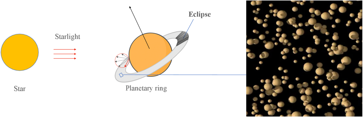
The idea behind this process revolves entirely around light. When sunlight hits a particle within a planetary ring, non-absorbed sunlight imparts a little “bump” onto a particle, ever so slightly altering its trajectory. At the same time, some of the sunlight is absorbed into the particle, which heats it up; light is soon re-emitted via thermal radiation, which, again, can slightly change the trajectory of these tiny particles. From a point on the surface of each ring particle (see rightmost side of Figure 2), the photons from this thermal radiation are all emitted in random directions; however, across the whole surface of the particle there is a net force! These tiny particles are spinning, and so the side just near “sunset” is hottest and emitting the most thermal photons. In this way, the pressure from the sunlight plus the thermal radiation of each particle imparts a net torque on the ring itself which changes the angular momentum of the ring.

diagram showing sunlight falling on Saturn and the planet casting a shadow on its rings

Figure 2: Starlight is the main source of light onto the particles that make up a planetary ring (right panel) though reflected light from the planet’s surface hits it too. This light “heats up” the ring and forms an asymmetry as the ring is eclipsed by the planet, which produces a net force. [Zhou et al. 2026]

What we described just then is essentially solar radiation pressure plus the Yarkovsky effect. It turns out that the net force from this process typically averages out to zero as the ring particles orbit around the planet. This assumes, though, that the sunlight is constantly shining on the ring. Stunning imagery of Saturn tells us that this isn’t the case, so what happens when we take into account the shadow cast on the ring from the planet? Today’s authors find that the net effect induces a positive change in angular momentum of the ring particles, which they call the eclipse–Yarkovsky effect.

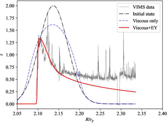
After today’s authors detailed all of the math involved in this process (and there is a lot), they put it into practice to try to help explain Saturn’s curious rings. Including the eclipse–Yarkovsky effect together with other known effects that drive ring evolution allowed them to reproduce the optical depth profile (how thick the ring looks) of Saturn’s A ring better than ever before (notably the sharp inner edge in Figure 3). On top of this, the effect provides another avenue for moonlet formation in the outer edges of ring systems as the positive torque from the effect drives material out toward and away from the Roche limit.

plot of optical thickness versus radius

Figure 3: The authors try to explain the current structure of Saturn’s A ring by initialising it with a Gaussian profile of optical thickness versus radius (black dot-dashed line) and evolving it for 81 million years under different effects. When viscous effects are included (blue dashed line), the ring spreads out, but it’s only when the eclipse–Yarkovsky (EY) effect is included (red line) that the model closely matches the observed data (grey line). [Zhou et al. 2026]

Undeniably useful for Saturn, the eclipse–Yarkovsky effect may also explain some other conundra in the solar system. Mars may have once had rings, which are thought to have eventually clumped together to form the inner moon Phobos. This idea is problematic, though, in that current models suggest there should still be some residual ring system around Mars even after Phobos formed. Enter the eclipse–Yarkovsky effect: being 100 times stronger for Mars than Saturn (due to its more intense incident sunlight), the effect may have driven out and dispersed that residual ring altogether. While the authors are currently looking into this possibility, the reintroduction of the eclipse–Yarkovsky effect has already shown great promise for our most beautiful ringed planetary neighbour.

Original astrobite edited by Wasi Naqvi.

About the author, Ryan White:

I am a first-year PhD student at Macquarie University in Australia, working mainly on binary/multiple systems with massive stars (Wolf–Rayets in particular!). Outside of study, I’m probably drinking coffee, baking, reading, or going for a run. You can also find me procrastinating on Bluesky @astroryan.bsky.social.

The post Shining a Light on the Shadowy Movements in Saturn’s Rings appeared first on AAS Nova.

June 8, 1625: The birth of Giovanni Cassini

8 June 2026 at 14:00

Giovanni Cassini was born in Perinaldo, in what is now Italy, on June 8, 1625. Early work on Jupiter and Mars’ rotational periods and the positions of Jupiter’s satellites led to an invitation to Paris and the Academie des Sciences by King Louis XIV; he became director of the Observatorie de Paris in 1671, andContinue reading "June 8, 1625: The birth of Giovanni Cassini"

The post June 8, 1625: The birth of Giovanni Cassini appeared first on Astronomy Magazine.

Now That’s Metal: How to Spot Stars That Have Swallowed Their Planets

3 June 2026 at 17:00

An illustration of an exoplanet about to be engulfed by its host star

Planets that get too close to their host stars are liable to be engulfed and consumed. New research explores how to identify stars that have had a planetary snack.

It’s Snack Time

Being a planet that closely orbits its star is dangerous, and various dynamical processes can draw a planet inward past the point of no return. When a planet vanishes beneath the surface of its host, it eventually disintegrates within the star, its atoms mixing into the blazing stellar soup.

This outcome is likely extremely common across the universe, and researchers have begun to see evidence for it: stars that appear to have absorbed angular momentum from their planets, white dwarfs with uncanny metals in their spectra, and stars with chemical abundances that don’t match those of their siblings. Now, in a recent publication led by Kaitlyn Lane (Vanderbilt University), researchers seek to find observational signatures of planetary engulfment of rocky exoplanets by main-sequence stars.

Modeling Engulfment

Lane’s team focused on main-sequence stars in the range of 0.5 to 1.4 solar masses, using one-dimensional analytical models to determine which of these stars will most readily display signs of having engulfed a planet. They simulated the stars as they consumed either an Earth-like planet or a super-Earth with the same composition as Earth but 15 times its mass.

illustration of a planet being engulfed by its star

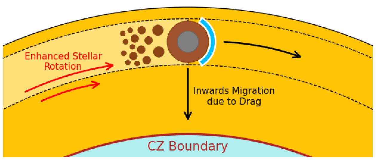
Diagram showing a planet being engulfed by its star and beginning to disintegrate before migrating inward. The boundary between the star’s outer convective zone (CZ) and inner radiative zone is shown. Click to enlarge. [Lane et al. 2026]

At the onset of the model, the engulfment is set to begin, the planet placed tangent to the star’s surface. The planets sink down and orbit just barely within their stars for 1–10 years, their solid surfaces slowly beginning to evaporate.

After that relatively lengthy phase, the process proceeds rapidly: as the planet inches deeper into its star, the drag forces grow stronger and the planet’s demise accelerates, with the planet disintegrating over the course of hours. In the last phase, the planet makes its final plunge and is destroyed in a half hour.

Signs of Planets Past

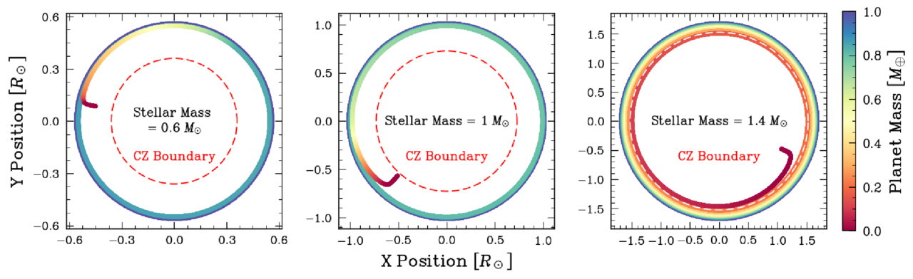
Lane’s team found that the planets tended to be destroyed fully within the outer convective layer of their stars, except in the case of the most massive stars studied here. For more massive stars, the outer convective zone is shallower than it is for the less massive stars, allowing a chunk of each planet to survive the passage through the convective zone to reach the radiative zone below.

simulation results showing planets disintegrating within their host stars

The trajectories of three example cases, showing how the planet loses mass as it spirals inward. In the 1.4-solar-mass case, part of the planet survives to reach the radiative zone, but the shallowness of the star’s convective zone means that the disintegrated planetary material is easier to observe. Click to enlarge. [Lane et al. 2026]

What this translates to, for the purposes of identifying planet-eating stars from afar, is that stars near the top of the mass range studied — from 1.0 to 1.4 solar masses — make the best targets. This is because the tell-tale planetary metals are not overly diluted within the stars’ relatively small convective zones, making these elements easier to detect. In terms of specific metals, the authors found that aluminum, calcium, and vanadium are the best signposts of planetary engulfment, with lithium also making the list.

While the authors acknowledge that there’s more work to be done — they plan to investigate the impacts of planetary engulfment on stellar structure more closely, for example — this work represents an important foray into identifying targets for future studies of stars that have eaten their planets.

Citation

“Observable Metal Pollution in Main-Sequence Stars: Simulations of Rocky Planets Engulfed by Stars in the 0.5 to 1.4 M⊙ Range,” Kaitlyn T. Lane et al 2026 ApJ 1003 67. doi:10.3847/1538-4357/ae5b9a

The post Now That’s Metal: How to Spot Stars That Have Swallowed Their Planets appeared first on AAS Nova.

The First Starspot Spectrum Revealed by JWST

2 June 2026 at 17:00

M-dwarf star with starspots

Editor’s Note: Astrobites is a graduate-student-run organization that digests astrophysical literature for undergraduate students. As part of the partnership between the AAS and astrobites, we occasionally repost astrobites content here at AAS Nova. We hope you enjoy this post from astrobites; the original can be viewed at astrobites.org.

Title: A Panchromatic JWST Spectrum of a Giant Starspot on the Fully Convective M Dwarf TOI-3884
Authors: C. A. Murray et al.
First Author’s Institution: University of Colorado Boulder
Status: Published in ApJ

We often picture stars as smooth, glowing spheres, as if they’ve been run through an Instagram filter. But real stars have spots: cooler, darker regions on a star’s surface caused by strong magnetic fields.

Annoyingly, these spots can seriously interfere with how we study exoplanet atmospheres.

How to Probe a Planetary Atmosphere

Planetary atmospheres are often probed through transmission spectroscopy. When a planet transits its star, some starlight passes through the planet’s atmosphere before reaching us. We can distinguish the light that has passed through the planet’s atmosphere by comparing the star’s light in transit versus out of transit. In doing so, we can isolate the atmospheric spectrum and look for absorption features of species like water or oxygen.

Easy, right?

How Starspots Get in the Way

Things get more complicated once we stop thinking of the star as if it’s been smoothed out by an Instagram filter. Starspots are cooler than the surrounding stellar surface, which means they emit a different spectrum. They are also constantly changing: new spots can form, old ones can disappear, and the star’s rotation carries them in and out of view. This changes things.

First of all, your star’s spectrum changes over time, which could mean that the star’s spectrum out of transit is not the same as the star’s spectrum during transit. On the other hand, the planet may transit across a starspot instead of a “normal” stellar region. In this case, the light we measure during the transit is affected by the spot, and it is no longer accurate to directly compare it with the overall stellar light outside the transit.

Ultimately, absorption features that we thought were from the planetary atmosphere could actually be coming from starspot contamination instead.

Starspot Models: Our Solution?

To deal with this, astronomers build starspot models, where they vary the spots in terms of the following:

  • The surface covering fraction: this parameter tells us how much of the stellar surface is covered in spots
  • The temperature contrast: this parameter tells us how much cooler (in ratio) the spot is compared to the rest of the stellar surface, and by proxy how much dimmer

These models are promising, but how do we know that we have chosen the right parameters?

A Unique Laboratory: TOI-3884

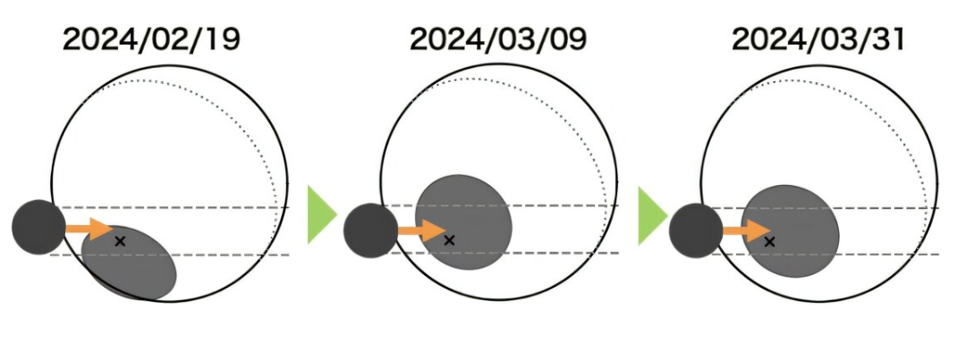
The TOI-3884 system is a unique laboratory for testing our starspot models. As seen in Figure 1, it has very convenient starspot geometry, with a large starspot located close to its pole. On top of that, we observe this star almost completely pole-on, which means that we always see this starspot, no matter how much the star rotates. To top this all off, the star hosts a close-in planet, which orbits the star from pole to pole.

Illustration of the TOI-3884 system

Figure 1: Illustration of the TOI-3884 system. The pole (and rotation axis) of the star is indicated with a black “x,” indicating that we see the star almost pole-on. The polar starspot is indicated in grey, and the transiting planet TOI-3884b is indicated in black. Different dates are shown, illustrating how the system evolves over the span of a few weeks. [Adapted from Mori et al. 2025]

The planet transits the star, and as it does so, it always passes over the polar starspot. This gives us a rare opportunity to probe the spectrum of a starspot. Similar to how we can use normal in/out of transit observations to probe a planetary atmosphere, we can now compare the observations during/after a “starspot transit” to probe the starspot region. Today’s authors do exactly this using six different transit observations from JWST.

So… How Good Are Our Models?

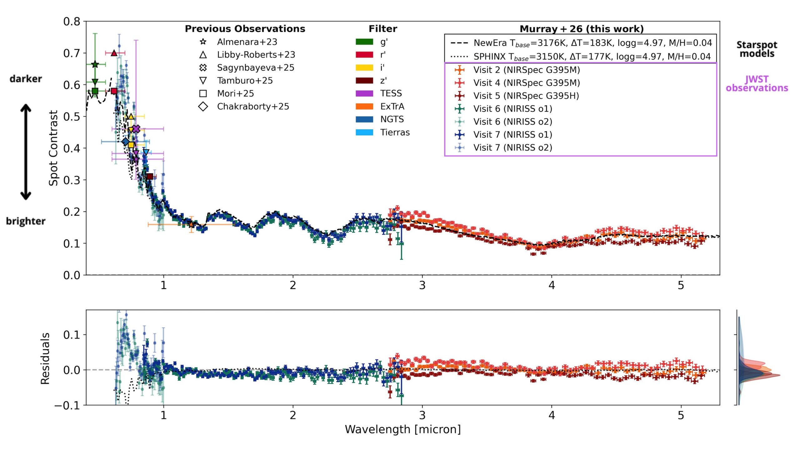
From the JWST observations, the authors extract a starspot spectrum for the first time. Figure 2 shows this as the spot contrast (how much dimmer the spot is than the surrounding stellar surface) plotted across different wavelengths. To see how well our models are doing, they compare this observed spectrum to two commonly used starspot models. The difference between the data and the models (the residual) is plotted in the lower panel.

spectrum of TOI-3884’s starspot.

Figure 2: The spectrum of TOI-3884’s starspot. The y-axis in the upper panel, the spot contrast, indicates how much dimmer the starspot is compared to the “normal” stellar surface. Different observations taken with JWST are indicated in different colored crosses, and other previous observations are overplotted in various other shapes. Model starspot spectra are shown in dashed or dotted black lines. The residuals between the model spectra and the JWST observations are shown in the bottom panel. [Adapted from Murray et al. 2026]

At wavelengths longer than about 1 micron, in the near-infrared regime, things look good! The residuals stay small, meaning the models do a solid job reproducing the observations. But move left into shorter wavelengths, in the optical regime, and the agreement quickly falls apart. The residuals grow, and it becomes clear that the models are missing something.

There’s still work to be done before we can confidently probe planetary atmospheres at optical wavelengths without worrying about stellar contamination, and this observed starspot spectrum provides a unique benchmark to test future starspot models. For now, the near-infrared remains a safer and more reliable window for planet atmosphere studies.

Original astrobite edited by Natalie Price.

About the author, Elise Koo:

I’m a PhD student at the University of Amsterdam, working to detect magnetic interactions between stars and their planets using radio and spectroscopic observations. Outside of research, I like to try out a variety of sports.

The post The First Starspot Spectrum Revealed by JWST appeared first on AAS Nova.

Life on the (Red) Edge

26 May 2026 at 17:00

Earth in visible and near-infrared light

Editor’s Note: Astrobites is a graduate-student-run organization that digests astrophysical literature for undergraduate students. As part of the partnership between the AAS and astrobites, we occasionally repost astrobites content here at AAS Nova. We hope you enjoy this post from astrobites; the original can be viewed at astrobites.org.

Title: Retrieving the Red Edge on Earth-Like Planets with Heterogeneous Clouds and Surfaces
Authors: Zachary Burr et al.
First Author’s Institution: Jet Propulsion Laboratory; ETH Zurich
Status: Published in ApJ

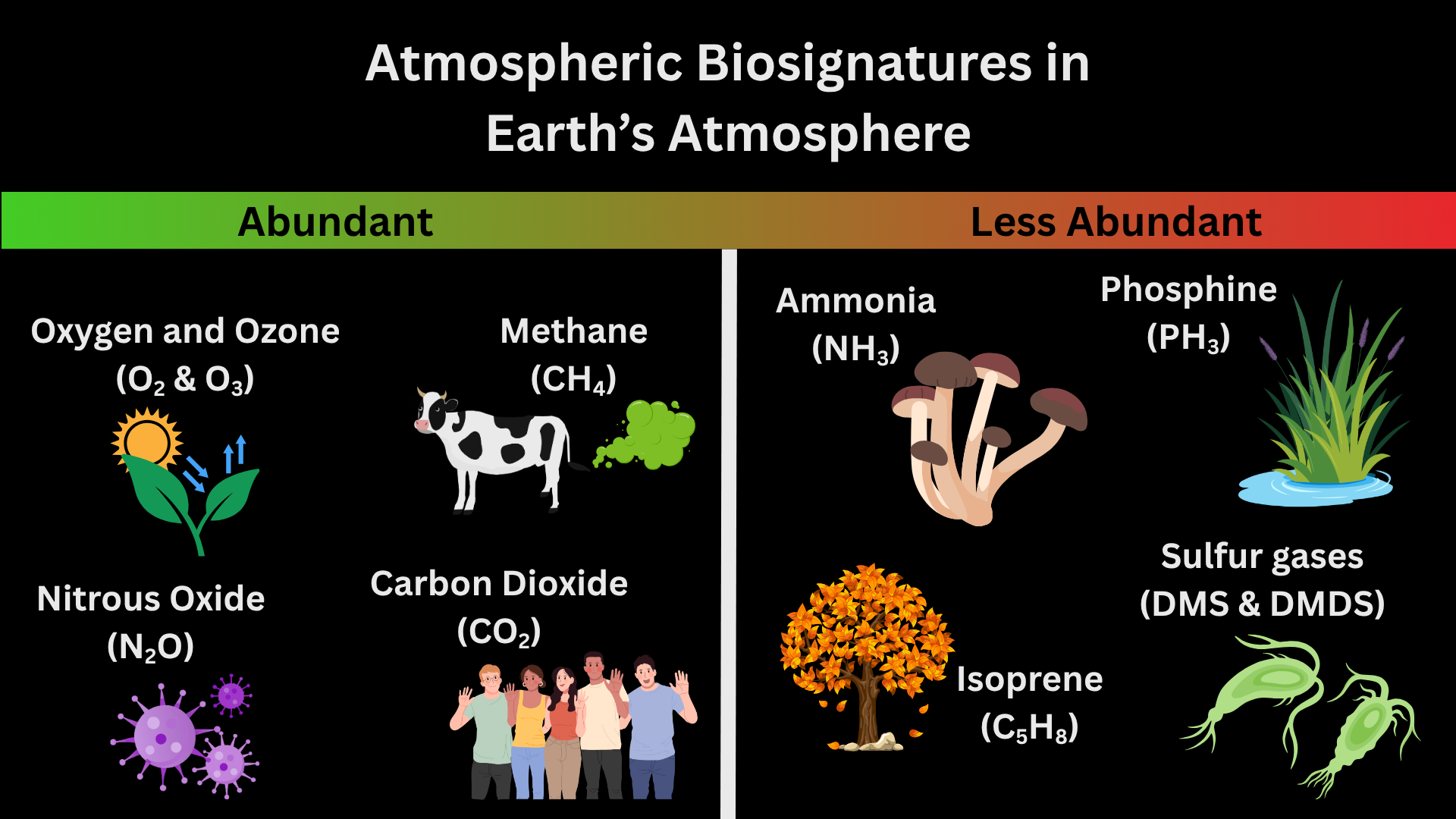
In the next 25 years, astronomers could find signs of life on other planets with the launch of the Habitable Worlds Observatory. Atmospheric signs of life, known as atmospheric biosignatures, are how astronomers currently search for life on other planets. Figure 1 shows examples of atmospheric biosignatures with pictures of each chemical’s origin on Earth. Before E.T. can phone home, though, we have to understand what chemicals make up a planet’s atmosphere. To do this, astronomers can use spectroscopy to observe a planet’s atmosphere in different wavelengths and measure the types and quantities of chemicals present.

biosignatures in Earth's atmosphere

Figure 1: Atmospheric biosignatures present in Earth’s atmosphere. More abundant biosignatures include oxygen and ozone (byproducts of photosynthesis in plants and bacteria) and nitrous oxide (byproduct of bacteria that don’t need oxygen to survive). Less abundant biosignatures include isoprene (released from the breakdown of leaves that have fallen from trees) and sulfur gases (byproducts of cyanobacteria). [Kaz Gary]

There are many ways to observe the spectrum of a planet, but the one you’re probably most familiar with is transmission spectroscopy. You can learn more about transmission spectroscopy of exoplanet atmospheres and how to model transmission spectra with these bites: 1, 2, 3. However, all of the current techniques for exoplanet spectroscopy (including transmission spectroscopy) measure the star’s light and how the planet affects the star’s light. This means it’s heavily dependent on how we model the star’s light to indirectly observe the planet’s light. The only way to take the spectrum of a planet directly is with direct imaging: the technique that the future Habitable Worlds Observatory will use to find signs of life in planetary spectra.

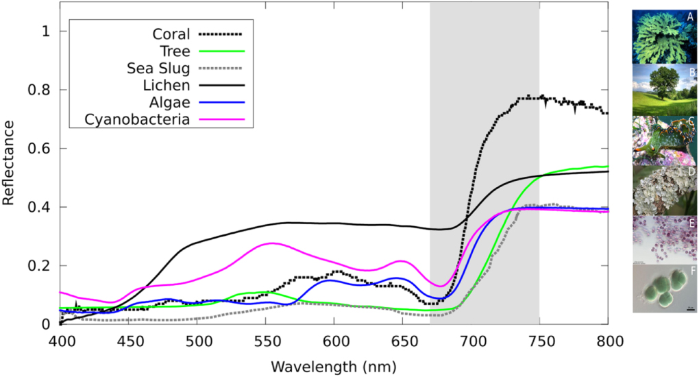
But are atmospheric biosignatures the only way to tell if life exists on other planets? Short answer: absolutely not. Let’s take Earth as an example. If we imagine Earth as a directly imaged exoplanet and take spectra of the light it reflects, you’ll find that around near-infrared wavelengths (~700 nanometers or just past the red part of the visible light spectrum), the light reflected off of Earth increases sharply. This sharp increase is called the vegetation red edge and is caused by plant and ocean life on Earth’s surface as shown in Figure 2. This is made possible because chlorophyll (the thing that makes plants green) absorbs nearly all visible light but reflects near-infrared light. The vegetation red edge is an example of a surface biosignature. In today’s article, the authors determine if the vegetation red edge will be visible in spectra of Earth-like exoplanets!

Spectra of different sources of the vegetation red edge

Figure 2: Spectra of different sources of the vegetation red edge on Earth. The vegetation red edge is highlighted in gray where the spectra rapidly increase and then level off beyond the visible light part of the spectrum. Each color represents a different source with pictures of each source on the right-hand side of the plot. [O’Malley-James and Kaltenegger 2019]

Snapshots

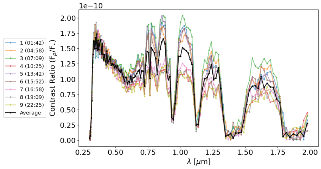
Planets rotate; that’s how we have morning, noon, and night in 24 hours guaranteed. This means that different parts of the surface will be visible at different times when we take spectra. Sometimes, we may see more ocean than land, other times not. To determine if the vegetation red edge would be visible at all points in Earth’s day, the authors simulated nine different spectra of modern-day Earth representing nine snapshots of Earth’s rotation. Additionally, they also simulated a time-averaged spectrum that shows an entire Earth day in one snapshot without the time variability. These spectra are shown in Figure 3.

Spectra of a directly imaged modern-day Earth at nine different times in its rotation

Figure 3: Spectra of a directly imaged modern-day Earth at nine different times in its rotation. The y-axis is the ratio of the planet’s signal to the star’s signal and the x-axis is wavelength in microns. Each color represents a time in UTC and the black curve represents the time-averaged spectrum. [Burr et al. 2026]

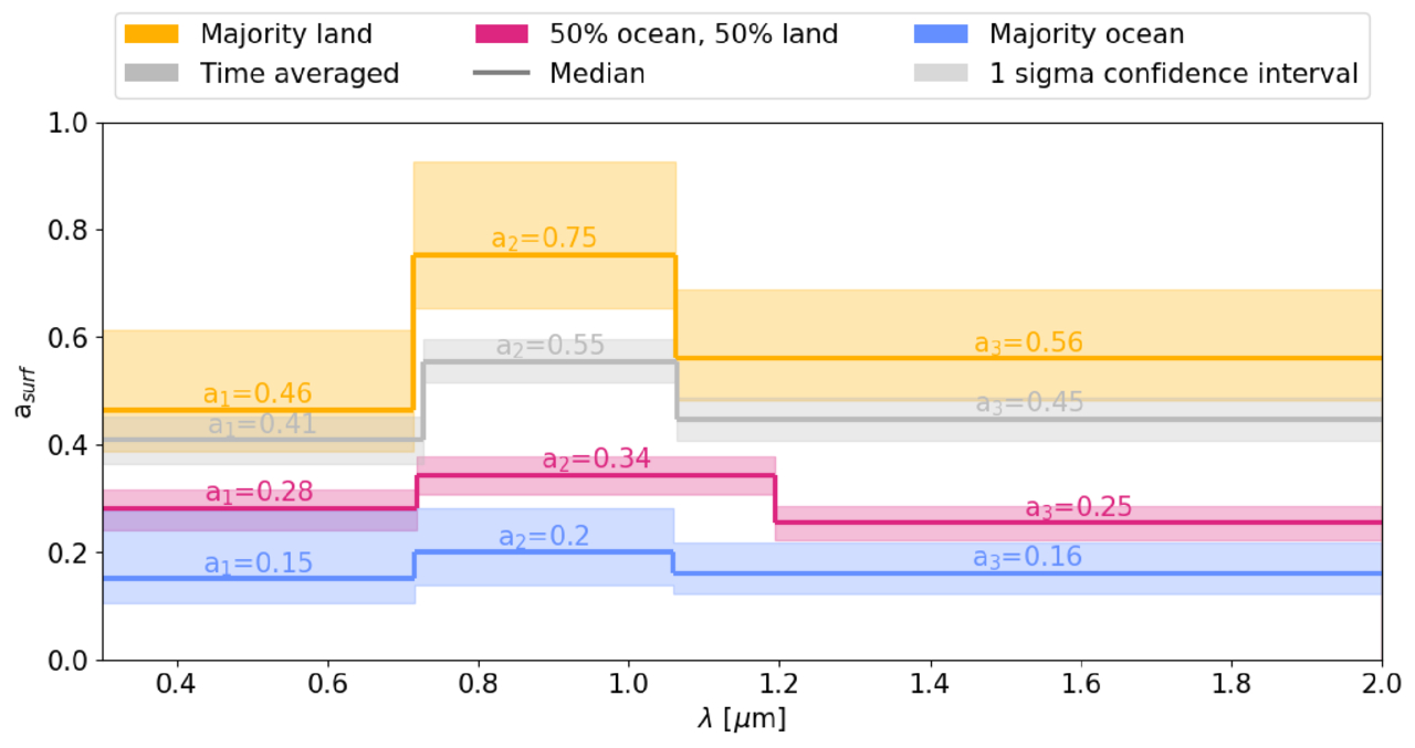
The authors then run retrieval models on all nine spectra to see if the vegetation red edge would be detectable in each spectrum, including the time-averaged one. Retrieval models take into account characteristics of the planet that would affect how light moves through its atmosphere, such as the atmospheric chemicals present and the surface gravity. They then use this information to generate possible spectral models that could fit the data. The best-fit model allows astronomers to infer what the atmosphere is made of and properties of the planet such as surface gravity. Because we are looking at Earth in visible light, much of the light from the planet is reflected. Typically, models of Earth-like planets in visible wavelengths only include atmospheric albedo: the measure of how reflective a planet’s atmosphere is. However, surface biosignatures can also be reflective as shown by the vegetation red edge. The authors use this to their advantage and introduce a surface albedo into their model that changes with the amount of desert, vegetation, and ocean visible on Earth’s surface at that time. They then further divide the nine spectra into three different types based upon the visible surface: majority land; 50% land, 50% ocean; and majority ocean. Check out the article online to see a cool animation of the Earth rotating and how the spectrum looks different at each time!

Arr! There Be… Vegetables?

After running the models, the authors were able to detect a sharp increase in the surface albedo value in every spectrum, including the time-averaged one. This result is shown in Figure 4. The authors take this result one step further in order to validate that the vegetation red edge is actually a result of surface variation of vegetation. They re-run models on each of their spectra but instead include a constant surface albedo instead of a time-varying one. This resulted in incorrectly measured radii, chemicals, and surface gravity in nearly all of the models. Without the vegetation red edge and surface features, the models could not accurately determine if life was present on Earth.

Retrieved surface albedos for the nine time-varying spectra

Figure 4: Retrieved surface albedos for the nine time-varying spectra. The surface albedo is broken down into three different values (a₁, a₂, a₃). Each of these values represents a change in the surface albedo at different wavelengths (i.e., how reflective the surface is at three different wavelengths). The nine spectra were broken down by the amount of surface that was visible at that time and color-coded for each category. The time-averaged spectrum is shown in gray. Each category of spectra was able to retrieve an increase in reflected light from the surface at vegetation red edge wavelengths. The spectra that had the majority land visible have the biggest increase in the surface albedo. This makes sense since the amount of visible vegetation is the largest with majority-land planets. [Burr et al. 2026]

For the first time (to the author’s knowledge), the vegetation red edge has been shown to be a promising and observable biosignature in Earth-like atmospheres. This study has also laid the groundwork for future work on other surface biosignatures and their potential impact on spectra of habitable planets. Confirming signs of life in multiple different ways, both on the surface and in the atmosphere, will finally allow astronomers to say we are not alone in the universe. In fact, life likes to live on the (red) edge!

Original astrobite edited by Madison VanWyngarden.

About the author, Kaz Gary:

I am a fourth-year PhD candidate at The Ohio State University with a passion for planets. My current work focuses on modeling exoplanet observations for the Habitable Worlds Observatory and understanding planetary atmospheres. Outside of research, I help develop planetarium shows and love all forms of science communication. In my free time, I enjoy playing tabletop RPGs, painting, watching terrible reality TV, and hanging out with my pet hedgehog.

The post Life on the (Red) Edge appeared first on AAS Nova.

Playing Pool with Planets

22 May 2026 at 17:00

artist's impression of hot Jupiter exoplanets

Each Jupiter-size planet in the galaxy falls into one of three distinct categories: hot, warm, or cold. A new study suggests that despite the apparent differences between these populations, they may have all formed from the same underlying dynamical process: a game of pool played at planetary scales.

A Diversity of Jupiters

Though our solar system has only one Jupiter-size planet, elsewhere in the galaxy we have found three different species of these massive gas giants. Cold Jupiters closely resemble their namesake and orbit far from their host stars; hot Jupiters are the opposite and are found whipping around their stars on extremely close-in orbits. In between these are the warm Jupiters, which tend to orbit in the intermediate space between 0.1 and 1.0 au.

A rendering of a star with lots of spots and flares with a planet in the foreground.

An artist’s depiction of a hot Jupiter. These planets orbit extremely close to their host stars, but likely got to their locations by scattering inward from more distant orbits. [NASA/JPL-Caltech]

Though these three populations are defined by their orbital distances, they differ from each other in other ways as well. For example, hot Jupiters almost never have nearby companions; if there are any other planets circling the same star, they’re usually far-out cold Jupiters. They can also orbit in pretty much any direction, including opposite the direction of their star’s spin, and are usually on perfectly circular orbits. In contrast, warm Jupiters often have friends nearby, are much more aligned with their stars’ spins, and can have modest eccentricities.

Given these differences, it’s often thought that each of these populations arrived at its current location through different dynamical processes and that the history of the warm Jupiters is likely quite different from the history of the hot Jupiters. However, a new study led by Julia Esposito (Georgia Institute of Technology) has proposed an alternative view. Maybe these populations, though they appear different now, were all created by the same process: planet–planet scattering.

Virtual Planetary Billiards

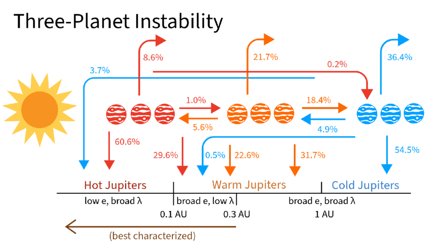
A cartoon of Jupiters at different distances from the sun with labelled arrows flowing inwards and outwards from each.

A schematic showing where different planets ended up as a function of where they scattered from during their evolution. Click to enlarge. [Esposito et al. 2026]

Esposito and collaborators set up 1,500 virtual planetary systems with three massive planets each, then simulated how the orbits evolved before probing the final configurations. In crucial contrast to previous simulation studies, the team initialized their Jupiters across a range of different distances and included the effects of tides sapping energy from orbits of planets that got too close to their host stars.

At the end of the simulation, the team surveyed the digital carnage. Almost every virtual system ended with only two planets after either ejecting one away from the star or having two planets collide. But, remarkably, the remaining two-planet systems looked tantalizingly similar to what we actually observe, with a mix of hot, warm, and cold Jupiters. Even more exciting, the end populations were highly correlated to where the violent scattering event took place.

For example, the warm Jupiters were almost all produced by “warm scattering” simulations, where the scattering took place between 0.1 and 1.0 au. The planets that survived the simulations and ended up as warm Jupiters matched all of the properties of the real warm Jupiter population: they had nearby companions, were moderately eccentric, and were mostly aligned with their stars. The hot Jupiters, meanwhile, were almost all produced by “cold scattering” events where the flybys happened far from the star and resulted in one planet hurtling inwards. These also matched all of the observed properties of real hot Jupiters.

The researchers concluded that planet–planet scattering can produce both the warm and hot Jupiter populations so long as you let the planets scatter from a variety of different distances. This exciting theoretical insight, if correct, would mean that astronomers could stop searching for different pathways to create each population. Happily, this model also provides testable predictions, and the authors lay out how the theory could be supported or disproven with additional data. Through virtual experiments like these, astronomers continue to build up an understanding of how the wide range of planetary architectures observed across the galaxy came to be.

Citation

“Unified Formation Channel of Hot and Warm Jupiters via Planet–Planet Scattering,” Julia Esposito et al 2026 ApJL 1003 L3. doi:10.3847/2041-8213/ae61b0

The post Playing Pool with Planets appeared first on AAS Nova.

Hunting for Exomoons Around a Lonely Planet

12 May 2026 at 17:00

illustration of an exoplanet and exomoon around a star

Editor’s Note: Astrobites is a graduate-student-run organization that digests astrophysical literature for undergraduate students. As part of the partnership between the AAS and astrobites, we occasionally repost astrobites content here at AAS Nova. We hope you enjoy this post from astrobites; the original can be viewed at astrobites.org.

Title: A Deep Search for Exomoons Around WISE 0855 with JWST
Authors: Mikayla J. Wilson et al.
First Author’s Institution: University of California, Santa Cruz
Status: Published in AJ

The “Moon”-umental Question

The solar system hosts hundreds of moons, ranging from volcanic worlds like Io around Jupiter, to icy objects like Enceladus around Saturn, to captured objects like Neptune’s retrograde moon Triton. Moons are essential to our model of how the solar system formed and also offer some of the best chances we have for finding life beyond Earth.

Astronomers also expect exomoons, or moons orbiting planets outside the solar system, to be abundant around other giant exoplanets. But how common are exomoons? How do they compare to the moons in our solar system?

In order to begin answering those questions, we must first detect an exomoon, which has proved difficult despite decades of searching by astronomers. Fortunately, JWST presents a new opportunity to uncover the exomoon population by looking at lonely free-floating planets as they drift through space.

Why Free-Floating Planets?

One proposed method for searching for exomoons is by looking for their transits in front of their host planets, characterized by the dips in brightness of the planet as the moon passes in front, blocking the planet’s light. Looking for exomoon transits around planets orbiting stars is quite difficult, as the bright starlight can easily drown out the small signals of exomoon transits. Free-floating planets solve this issue by removing the star entirely, increasing our sensitivity to such detections. (See this bite for a good review.)

The authors of today’s article directed the exomoon hunt towards the free-floating WISE J085510.83-071442.5 (or WISE 0855). It has the prestige of being the coldest known brown dwarf (250–285K) while also sitting at a relatively low mass (3–10 Jupiter masses). Notably, it is also one of our closest neighbors at a distance of only 7.4 light-years, making it ideal for high-precision observations despite its faintness. Even though brown dwarfs are technically distinct from planets, the authors opt to refer to companions around WISE 0855 as moons given WISE 0855’s “planetary-mass” status. (It’s complicated…)

Repurposing JWST Data… for Moons!

The JWST observations used in this study contain 11 hours of near-infrared (2.87–5.27 microns) time-series spectra originally intended to study water clouds and weather on WISE 0855. Time-series brightness monitoring can also be used for transit searches, which the authors take advantage of.

One complication is that WISE 0855 is variable, meaning its intrinsic brightness changes over time. Variability is likely driven by clouds and other dynamic processes within its atmosphere. So how do the authors distinguish between a passing moon and a turbulent atmosphere? The key idea is that variability is wavelength dependent, meaning that the brightness of WISE 0855 will fluctuate differently depending on the observed wavelength. In contrast, transits are “gray,” meaning that the same amount of light is blocked at all wavelengths, producing a consistent feature across the entire spectrum.

Finding Moons with Statistics!

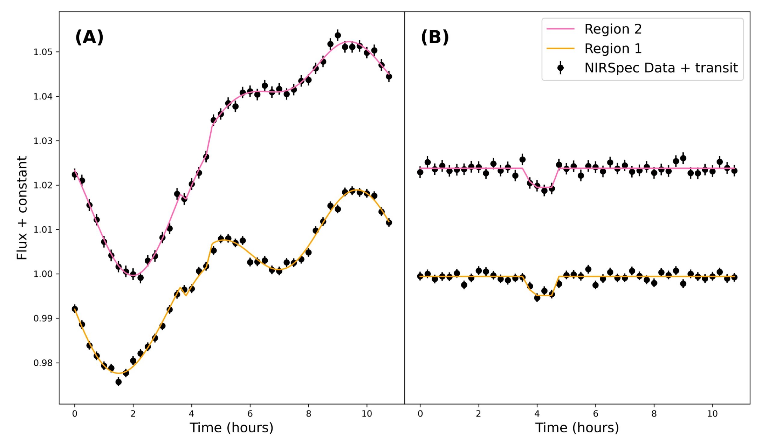
The authors apply this idea and pick out two wavelength regions of WISE 0855’s spectrum that contain two distinct variability patterns, which should both contain an identical moon transit signal (if present). They then generate a light curve (how brightness changes over time) for these two regions (see Fig. 1).

WISE 0855 light curves

Figure 1: (A) Light curves from two selected wavelength regions of WISE 0855’s spectrum with injected transit signals. Also plotted is the best-fit Gaussian processes + transit model for the two light curves. (B) Light curve data after subtracting the Gaussian processes portion of the best-fit model, revealing the example injected transit signals. [Wilson et al. 2025]

To appropriately model the variability, the authors employ Gaussian processes, a flexible tool that can model complex, quasi-periodic signals like atmospheric variability. They compare fits from two types of models:
  • Gaussian processes–only model: Assumes that all observed variability is intrinsic to the planet itself
  • Gaussian processes + transit model: Includes a simple trapezoidal exomoon transit signal that is simultaneously fit in both light curves

Using Bayesian evidence (a measure of how well each model explains the data), they determined which model was favored. So, what do they find?

The Bad News and the Good News

Based on Bayesian evidence, the authors conclude that there are no statistically significant detections of exomoons in the data. The results suggest very weak evidence for a ~0.53-Earth-radius moon at a wide separation from WISE 0855 — an unlikely scenario given that transit probability decreases at greater separations (and therefore longer orbital periods).

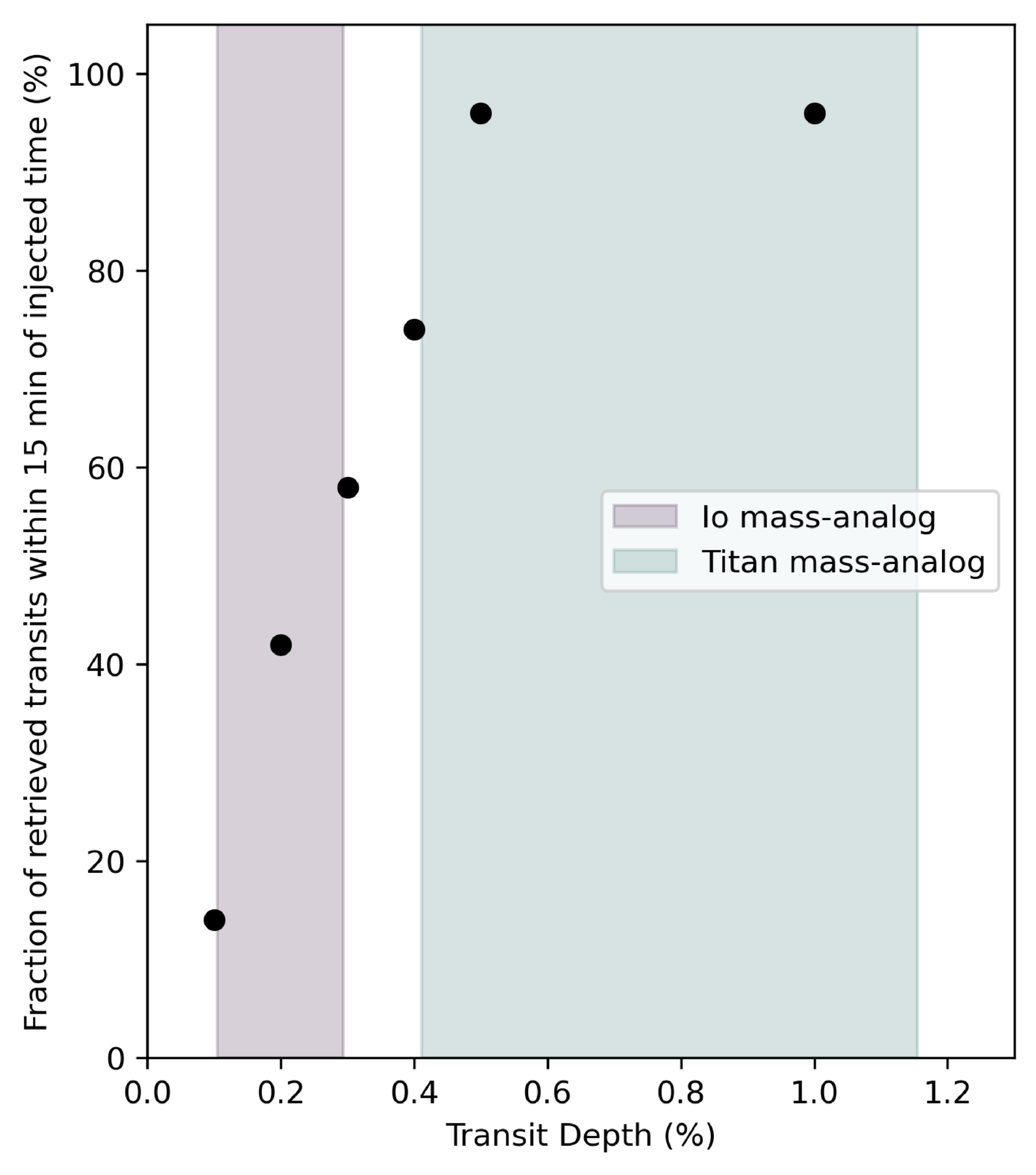
Yet, the study goes further: What kinds of moons is JWST able to detect, if any? To answer this, the authors performed injection and recovery tests, where they injected artificial transit signals of varying depths (exomoon sizes) into the data and tested how well their models were able to recover them (results shown in Fig. 2). They find that JWST is capable of detecting 96% of transits with depths ≥0.5%, equivalent to a Titan-like moon. Smaller Io-like moons were also detectable more than half of the time. This means that if a Titan analog had actually transited during these observations, we would almost certainly have seen it!

plot of successful detections of injected transit signals

Figure 2: Results showing the number of successful detections for the transit injection and recovery tests. Fifty transit injections are done for transit depths of 1%, 0.5%, 0.4%, 0.3%, 0.2%, and 0.1%. The transit depths represent different exomoon sizes, with the shaded regions representing Io-like and Titan-like moons. [Wilson et al. 2025]

JWST will continue to gather more time-series data of free-floating planets, brown dwarfs, and directly imaged exoplanets, each providing a new opportunity to help us better understand the moon population outside of our solar system. We’re still waiting for the first confirmed exomoon, but when that transit finally happens, we know that JWST will be ready.

Original astrobite edited by Kelsie Taylor.

About the author, Jared Bull:

I am a 2nd-year PhD student at Johns Hopkins University. I study brown dwarf variability and am interested in using time-series observations to uncover dynamic processes within their atmospheres. In my free time I like to read, cook, and do astrophotography.

The post Hunting for Exomoons Around a Lonely Planet appeared first on AAS Nova.

Characterizing the Atmosphere of Exoplanet WD 0806b with JWST

3 April 2026 at 17:00

gas giant orbiting white dwarf

Orbiting a white dwarf, the exoplanet WD 0806b is the subject of a recent study using JWST to measure the atmospheric conditions governing the planet.

Directly Imaged Exoplanet WD 0806b

Most of the 6,000 and counting exoplanets discovered thus far have been detected due to their impacts on their host star — passing in front of the star and causing it to dim, or gravitationally tugging on the star and causing it to wobble. On rare occasions, though, astronomers have been able to catch the exoplanet itself through direct imaging. Directly imaged exoplanets offer key insights that cannot be obtained through indirect detection methods. Luminosity measurements and spectral emission features allow astronomers to more directly measure planet mass, radius, and composition otherwise inferred from the host star.

WD 0806b system

NIRCam image showing host star WD 0806 circled in orange and the location of exoplanet WD 0806b marked by the orange arrow. [Lew et al 2026]

Included in the about 90 distant planets that have posed for a picture is WD 0806b, a rare exoplanet companion trotting around a white dwarf at an orbital distance of 2,500 au (50 times the distance from the Sun to the Kuiper belt!). Originally discovered with the Spitzer Infrared Array Camera in 2011, WD 0806b is the second-coldest directly imaged exoplanet to date. With JWST’s high-precision photometric and spectroscopic capabilities, WD 0806b provides a unique opportunity to probe the atmospheric chemistry of cold giant planets and take steps toward understanding the co-evolution of white dwarfs and their surviving exoplanets.

WD 0806b’s Atmospheric Abundances from JWST

Aiming to characterize the physical properties and atmospheric composition of WD 0806b, Ben W.P. Lew (Bay Area Environmental Research Institute; NASA Ames Research Center) and collaborators used JWST’s Near-Infrared Camera (NIRCam) and Near-Infrared Spectrograph (NIRSpec) to obtain high-resolution imaging and spectroscopy of the exoplanet. Combining these observations, prior lower-resolution observations, and evolutionary planet models, the authors estimated the physical properties of WD 0806b including mass, radius, surface gravity, and effective temperature.

WD 0806b spectrum

NIRSpec spectrum of WD 0806b with best-fit model spectra overlaid. [Lew et al 2026]

From the derived physical properties, the authors modeled the NIRSpec spectrum to estimate molecular abundances and elemental abundance ratios in the atmosphere of WD 0806b. They obtained measurements of multiple molecules including carbon dioxide, carbon monoxide, and ammonia; these molecular abundances offer the opportunity to test chemical equilibrium and disequilibrium as well as eddy diffusion, or bulk mixing, in the planet’s atmosphere. The authors developed a novel chemical analysis framework to determine how bulk mixing varies with altitude in WD 0806b and reported the first observational evidence that mixing becomes weaker at higher altitudes in exoplanet atmospheres. This result points to the need for future studies exploring the impact of these chemical processes on spectra and photometry, which are essential to characterizing cold giant planets.

This study highlights how high-precision JWST data can reveal a rich collection of atmospheric conditions, chemical composition, and physical processes occurring in cold giant planets. With such a wide orbit from its host white dwarf, WD 0806b serves as an interesting case study for how giant planet composition may reflect the formation and evolutionary history of the overall system. Future observations of and comparisons to similarly cold giant planets will further uncover how atmospheric characterization may fit into our understanding of exoplanets and their histories.

Citation

“JWST Spectral Retrieval of Cold Directly Imaged Planet WD 0806b and the First Measurement of Altitude-dependent Kzz in Exoplanet Atmospheres,” Ben W.P. Lew et al 2026 AJ 171 227. doi:10.3847/1538-3881/ae4747

The post Characterizing the Atmosphere of Exoplanet WD 0806b with JWST appeared first on AAS Nova.

Getting a Peek of Kitt Peak National Observatory

23 January 2026 at 17:00

KPNO

After AAS 247 in Phoenix, Arizona, AAS Nova Editor Kerry Hensley and I had the chance to travel about 150 miles south for a tour of Kitt Peak National Observatory.

A Window into Kitt Peak

Located 60 miles southwest of Tucson, Kitt Peak National Observatory (KPNO) resides on a mountain top within the Tohono O’odham Nation reservation. Founded in 1958, Kitt Peak is home to nearly two dozen active telescopes ranging in wavelength coverage and scientific objectives. Ronald Proctor, Lori Allen, and Jacelle Ramon-Sauberan, all serving in crucial roles for the observatory, led our tour around the mountain.

Windows Center Lobby

The Windows On the Universe Center’s lobby exhibit displaying the Tohono O’odham language with words describing the land and astronomy. Jacelle Ramon-Sauberan, the Tohono O’odham Nation Education Liaison, is seen to the left. [KPNO/NOIRLab/NSF/AURA/R. Proctor; CC BY 4.0]

Our visit began in the new Windows on the Universe Center — the first science center inside of a telescope. Situated inside the retired McMath-Pierce Solar Telescope, the Windows Center takes visitors through exhibits exploring the universe, the telescope’s original control room, and the observatory’s connection to the Tohono O’odham Nation.

The center’s lobby introduced visitors to the beautiful land KPNO calls home. Working with Tohono O’odham linguists, Jacelle, the observatory’s Tohono O’odham Nation Education Liaison, curated the lobby exhibit that features the native language and the Nation’s connection to astronomy and the observatory. The science center serves as an educational resource and place of cultural exchange, expanding the relationship between the observatory and the Tohono O’odham Nation. 

Astronauts

Apollo astronauts in the control room of the McMath-Pierce Solar Telescope in 1964. [United States Geological Survey; CC BY 4.0]

After walking through an introduction to the universe exhibit, visitors enter the original control room of the telescope. Mirrors across the room’s ceiling focus the Sun’s light onto table screens where visitors can observe the Sun in real time without burning their eyeballs. In addition to observing the Sun, the solar telescope allowed astronauts in the 1960s to view a projection of the Moon’s surface and plan their landing site for the Apollo 11 mission. Visitors can stand in the same place and witness the instruments that made the moon landing possible.

At the end of the Windows Center is a Science On a Sphere Theater — a spherical display system that allows visitors to see planets, stars, moons, and even large-scale structures of the universe in 3D. Featuring multiple programs, the theater takes visitors through the universe and displays data collected right there on the mountain!

WIYN

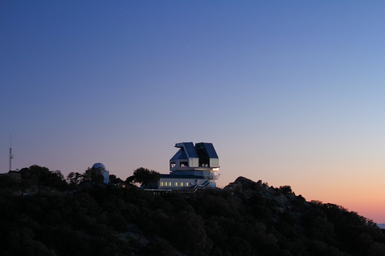
The WIYN 3.5-meter telescope at sunset. [KPNO/NOIRLab/NSF/AURA/P. Marenfeld; CC BY 4.0]

A WIYN for Exoplanetary Science

Though not typically open to the public for tours, our next stop took us to the WIYN 3.5-meter telescope. This telescope is operated and owned by the WIYN Consortium, a partnership between the University of Wisconsin, Indiana University, NSF’s NOIRLab (National Optical-Infrared Astronomy Research Laboratory; formerly NOAO), Pennsylvania State University, and Princeton University. Operating since 1994 with a strong collection of instruments, WIYN has observed galaxies near and far, stars across their lifetimes, and exoplanets tugging on their host stars.

Lexi at WIYN

Me, Lexi Gault (AAS Media Fellow), in front of the WIYN 3.5-meter telescope. I have used WIYN’s SparsePak spectrograph to collect data for my dissertation research! [AAS Nova/Kerry Hensley]

WIYN’s newest instrument, NEID (pronounced “NOO-id”), has been advancing exoplanetary science since its first light in early 2020. Derived from the word meaning “to see” in the Tohono O’odham language, NEID is a high-resolution spectrograph that uses the radial velocity method to detect exoplanets. As a planet orbits its host star, its gravitational pull induces a wobble in the star, and NEID can detect these wobbles with unprecedented precision. This instrument allows astronomers to find exoplanets that were previously undetectable.

The partnership between public and private universities and a government institution was the first of its kind. Through this consortium, hundreds of undergraduate and graduate students have conducted research with WIYN, and the telescope’s suite of instruments have enabled early career astronomers to explore the universe both near and far.

Mysteries of Dark Energy at Mayall

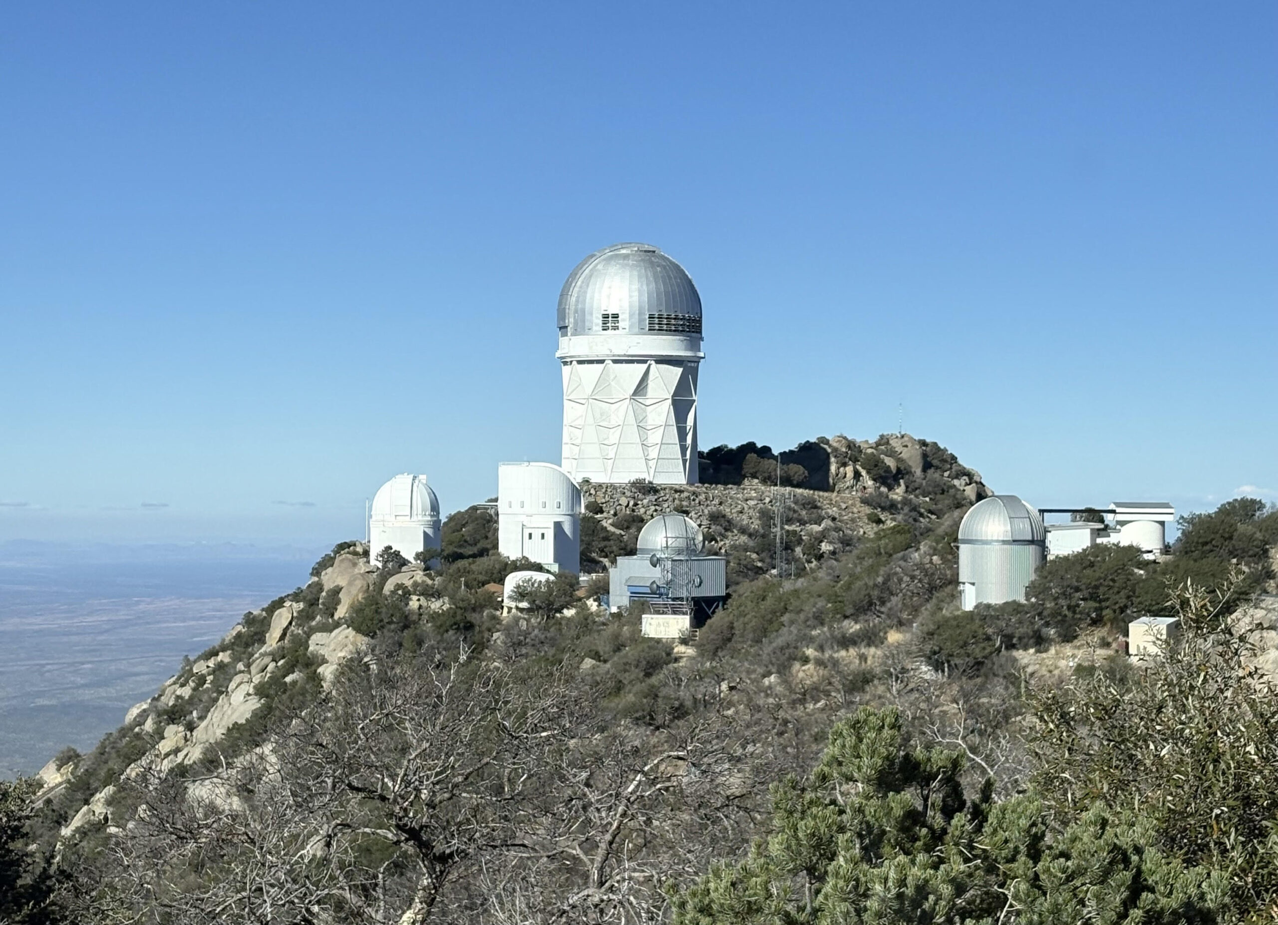
We concluded our tour at the Mayall 4-meter Telescope, the tallest telescope dome on the mountain at a staggering 18 stories high. This iconic telescope saw first light in 1973, and at the time, was the second-largest (in diameter) telescope in the world. Originally built for wide-field optical and infrared studies of the universe, the Mayall has enabled decades of critical scientific research.

Mayall dome

The Mayall dome across the mountain as seen from inside the WIYN dome. [AAS Nova/Lexi Gault]

Mayall is now home to the Dark Energy Spectroscopic Instrument (DESI), the most powerful multi-object survey spectrograph in the world. The DESI survey measures the impact of dark energy on the expansion of the universe through creating the largest ever 3D map of the universe. Mapping the distances to hundreds of millions of galaxies, DESI has revolutionized cosmology and enabled groundbreaking research into the origins of the universe. 

From the telescope’s massive dome, to the busy DESI control room, to the gallery floor with a nearly 360 degree view of the surrounding desert, the Mayall offers visitors a unique glimpse into Kitt Peak’s history and its future. While WIYN is a hidden gem, the Mayall 4-meter Telescope is open to the public for tours daily, so you can experience the exciting era of research and discovery at KPNO. 

Visit Kitt Peak

Interested in getting a peek yourself? KPNO is open to the public daily with multiple tour types to choose from, including both daytime and nighttime visits! Plan your visit to Kitt Peak here.

The post Getting a Peek of Kitt Peak National Observatory appeared first on AAS Nova.

Are Water Worlds Just Made of Soot?

20 January 2026 at 17:00

illustration of K2-18b

Editor’s Note: Astrobites is a graduate-student-run organization that digests astrophysical literature for undergraduate students. As part of the partnership between the AAS and astrobites, we occasionally repost astrobites content here at AAS Nova. We hope you enjoy this post from astrobites; the original can be viewed at astrobites.org.

Title: Soot Planets Instead of Water Worlds
Authors: Jie Li et al.
First Author’s Institution: University of Michigan
Status: Published in ApJL

They Might Be Planets with a Lot of Water…

Since the discovery of PSR B1257+12 c and d in 1992 and  51 Pegasi b in 1995, we have found evidence for thousands of planets in other star systems. One of the most striking things (aside from how common planets seem to be) is how many of them are so unlike anything we had imagined we would find. Our growing list of exoplanets includes a truly remarkable variety of types, from cold rocky planets smaller than Earth to scorching hot giants bigger than Jupiter.

However, one category of planets is particularly interesting: the sub-Neptunes. These planets, smaller than Neptune but larger than Earth, are characterized by their low densities, which suggests they could be dominated by water or volatile-rich atmospheres. What makes sub-Neptunes so intriguing is that we don’t have a clear counterpart for them in our own solar system. As such, we don’t really know a lot about them other than there seem to be a lot of them out there.

Although these planets are sometimes theorised to be rocky worlds with large hydrogen–helium envelopes, they have alternatively been considered as water worlds, i.e., worlds with giant planet-wide oceans thousands of kilometres deep. The thinking goes that since water ice appears to be abundant beyond the snow line, water worlds would be a natural consequence of planet formation. And if these planets exist, some might host a temperate liquid ocean with the conditions for life.

…or They May Just Be CHON(ky)

However, today’s article suggests that these supposed water worlds may not be as wet as we think they are. They may instead be rich in what are called refractory carbonaceous materials. This term describes solids rich in carbon, hydrogen, oxygen, and nitrogen, or CHON. It is a bit of a mouthful and is often just referred to as “soot,” but it is important to remember that it is different from the black stuff you would find in ye old chimney. Soot, in this case, is a major component of comets. We know that this type of material is present around planet formation, as protoplanetary dust contains not just silicates (rock) and water ice but also a significant amount of CHON, and comets are leftovers from this dust.

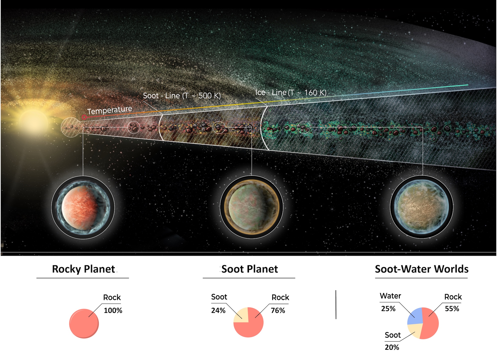
Soot is stable and remains in the solid state to much greater temperatures (∼500K) than water ice (∼160K), so the authors argue that there should be regions in the protoplanetary disk where planets accrete both rock and soot but little water. They define a “soot line” akin to the snow line and look at three archetypical planets that may form, shown in Figure 1.

illustration of rocky planets, soot planets, and soot-water planets based on their formation location

Figure 1: Illustration of a protoplanetary disk and three chemically distinct planet types that may form as the distance from the host star increases. Close in, the temperature in the disk is too high for volatiles to exist in the solid state, but farther out, the temperature drops to allow for water to freeze into ice beyond the water ice line, also known as the snow line. Between the two regions lies another where it’s cool enough for carbonaceous materials or “soot” to avoid destruction via thermally driven reactions. Depending on where planets form, they may contain a varying amount of astrophysical soot. [Li et al. 2026]

Inside the soot line, planets would be rock-rich worlds with low carbon or water content (e.g., terrestrial planets) because it is just too hot for any soot to stay together. Beyond the soot line but before the snow line, you would find carbon-rich rocky worlds (soot planets). They have low water content, as it is still too hot for water ice to exist, but these planets are rich in CHON. Beyond the snow line, a combination of rock/carbon/water worlds becomes possible, here labelled as soot-water worlds. The authors note that even though the last one has a significant fraction of water, it is distinct from traditional “water worlds” because it includes a significant component of hydrocarbon-rich material. Again, it is also important to remember that a soot world wouldn’t mean a black powder ball hanging in space, but rather a world that is composed of a lot of CHON, like Saturn’s moon Titan.

What Do the Models Say?

The authors got down to modelling planet compositions based on both observations of protoplanetary disks and the distribution of solid materials found in comets.

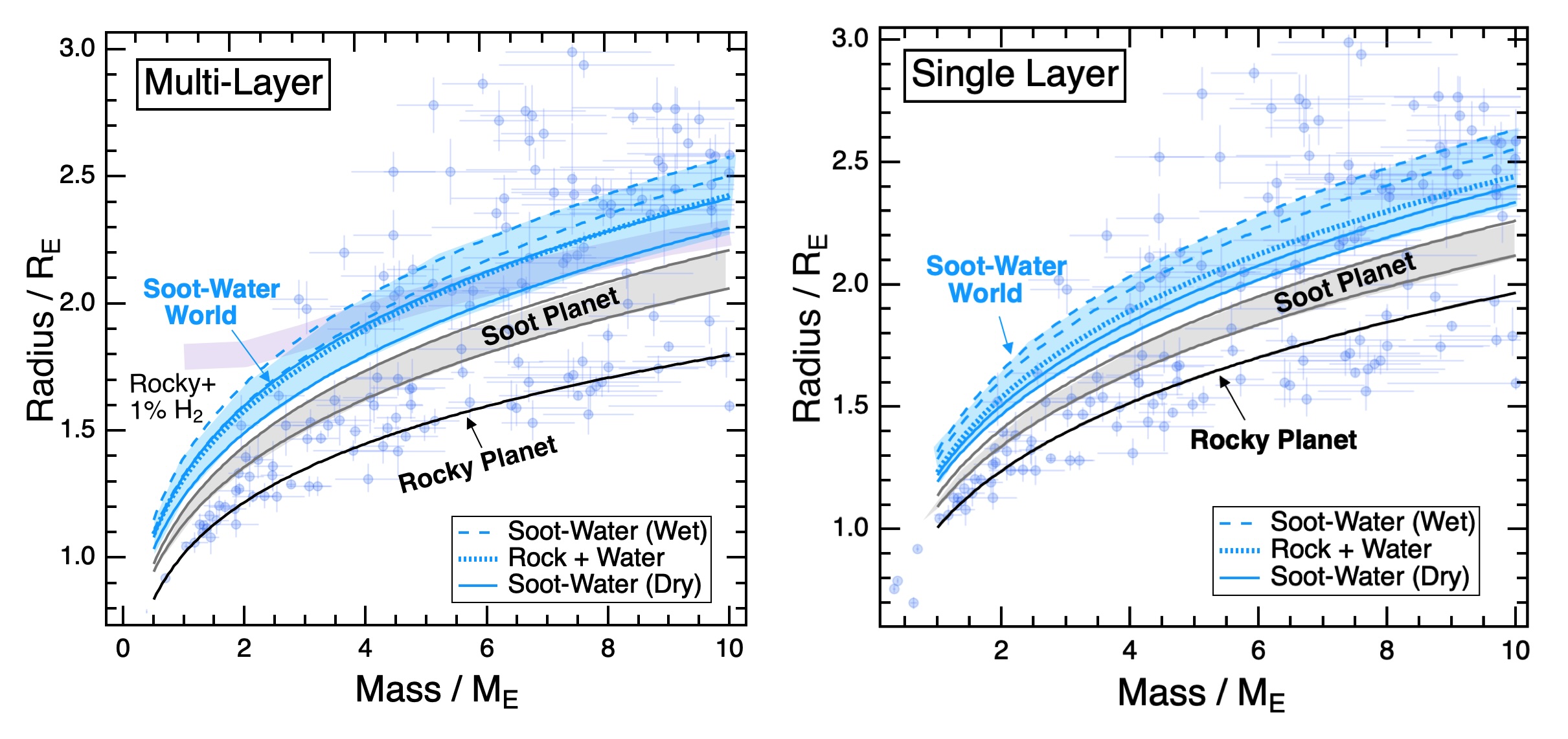
They considered two model planets. One is fully stratified, i.e., with a metallic core enclosed in a silicate mantle overlain by a hydrocarbon-rich layer and then a water-ice surface layer. The other, a single-layer mixed planet, is a hypothesised scenario where iron, silicate, soot, and water are fully mixed throughout the planet as a result of exotic chemistry from the high temperature inside the sub-Neptune planet. They expect any potential real planets to lie somewhere between the two extremes. The mass–radius relations for these models can be seen in Figure 2, where they are also compared to a number of known exoplanets, of which several fall within the models’ parameter spaces.

Mass–radius relations for model Earth-like rocky planets

Figure 2: Mass–radius relations for model Earth-like rocky planets (black curves), soot planets (gray bands), and soot-water worlds (blue bands). On the left are multi-layer planets, while on the right are single-layer planets. Overlaid are a number of exoplanets along with their respective uncertainties. Also shown as dashed lines are models for Earth-like planets with 50% rock and 50% water. These fall squarely within the same region as soot-water worlds, making the two indistinguishable from each other. [Li et al. 2026

A particularly interesting result that the authors note is that the predicted mass–radius relationship for the water worlds, which incorporates soot, is similar to that predicted previously for a 50% water planet with no carbon. That is, if you base your interpretation on the mass–radius relationship alone, it is impossible to distinguish between a world made of rock and water and a water-rich planet that incorporates a significant amount of soot.

We Might Have a Telescope That Can Help

How might we break through this impasse? Well, because significant fractions of methane and other simple hydrocarbons are expected to be released from the interior, the soot-rich planets may feature methane-rich atmospheres. These may naturally lead to the formation of hydrocarbon hazes, akin to the tholins in Titan’s atmosphere.

Looking at the atmospheres of exoplanets is one of the main mission goals of JWST. Many of the spectra from sub-Neptunes have so far been featureless, which may indicate the presence of clouds or photochemical haze. The telescope also has the ability to detect carbon-bearing species in the atmospheres of other sub-Neptunes, like with the discovery of CO2 and CH4 in the atmospheres of K2-18b and TOI-270d. Although these planets currently orbit interior to the soot lines of their respective stars, they may have originally formed farther out and later migrated inward during their evolution. Of particular interest is TOI-270d. Aside from also showing signs of water, it has a carbon-to-oxygen ratio that is moderately high for the planet, hinting that it could be a world with a considerable amount of soot.

The presence of soot may have significant implications when it comes to habitability. The planet’s core may be rich in diamond, which would impede the movement of volatiles in the mantle. This would make it challenging for the planet to generate a magnetic field and thus leaving any potential life vulnerable to cosmic radiation. However, they could also be abundant in methane and other volatile organic compounds, substances thought to be crucial for the development of prebiotic chemistry. Regardless, it is interesting that there might be something out there that is not so unlike something we know from our own solar system, a hazy supersized Titan. While the frigid moon is unlikely to show signs of life, a temperate soot-water world might be one place to look in the future.

Original astrobite edited by Sowkhya Shanbhog.

About the author, Kasper Zoellner:

I have a Master of Science in astronomy and I am currently working towards a PhD in physics and educational science. My greatest passion is the search for exoplanets and how stellar variability may influence the possibility of life. I am also interested in science outreach, education and discussing what sci-fi novel to read next!

The post Are Water Worlds Just Made of Soot? appeared first on AAS Nova.

Selections from 2025: Could Earth Detect Earth?

30 December 2025 at 17:00

Earth

Editor’s Note: For the remainder of 2025, we’ll be looking at a few selections that we haven’t yet discussed on AAS Nova from among the most-downloaded articles published in AAS journals this year. The usual posting schedule will resume January 2nd.

Earth Detecting Earth: At What Distance Could Earth’s Constellation of Technosignatures Be Detected with Present-day Technology?

Published February 2025

Main takeaway:

In a collaborative effort between the Search for Extraterrestrial Intelligence (SETI) Institute and the Penn State Extraterrestrial Intelligence Center, Sofia Sheikh (SETI Institute) and team turned inward to expand the search for intelligent life in the universe. Right here on Earth, humans have created a laboratory of technological signatures that can be detected from space — if another Earth-like civilization is out there, could they detect us? Using theoretical modeling, the authors determined the reaches of various human technosignatures such as radio transmissions, optical and infrared emission, satellites, and other probes sent into space. They found humanity’s strongest signals, radio transmissions, could be detected as far as 12,000 light-years away.

Why it’s interesting:

Scientists search for intelligent civilizations by hunting for signs of technology — signals or patterns that natural phenomena cannot explain. While we cannot expect other intelligent life to look exactly like Earth’s, many SETI projects have surveyed the skies for hypothetical signals far exceeding humanity’s own technological advancements. Taking a step back, Sheikh and collaborators considered where human technology is currently and what present-day instrumentation could pick up on if we were to search for ourselves. This “Earth detecting Earth” paradigm recenters the search for intelligent life and provides a multiwavelength framework for understanding the detectability of technology on far-away worlds.

Maximum detectability of Earth's technosignatures.

Maximum distances that Earth’s technosignatures could be detected by current technology. Click to enlarge. [Sheikh et al 2025]

Earth’s constellation of technosignatures:

What exactly are Earth’s many technosignatures, and how far could our current technology detect them? The most prominent and farthest detectable signal comes from radio transmissions. As the authors noted, these signals come from multiple sources: targeted radar transmissions used to characterize planets and asteroids, radio transmissions used to communicate between space probes and ground stations (e.g., space telescopes, Mars rovers, etc.), and radio leakage from Earth’s communication systems like cell towers and broadcasting stations. Additionally, there are atmospheric technosignatures from air-polluting compounds, optical and infrared emission from cities, targeted lasers from telescopes, and interplanetary and interstellar probes sent into space. All of these combined create a constellation of technosignatures detectable across a range of distances from Earth. This study underscores the importance of assessing Earth’s technology and detection capabilities, and repeating this type of study as technological advancements continue will enhance the search for intelligent life.

Citation

Sofia Z. Sheikh et al 2025 AJ 169 118. doi:10.3847/1538-3881/ada3c7

The post Selections from 2025: Could Earth Detect Earth? appeared first on AAS Nova.

Selections from 2025: JWST Searches for an Atmosphere on TRAPPIST-1e

26 December 2025 at 17:00

illustration of the TRAPPIST-1 system

Editor’s Note: For the remainder of 2025, we’ll be looking at a few selections that we haven’t yet discussed on AAS Nova from among the most-downloaded articles published in AAS journals this year. The usual posting schedule will resume January 2nd.

JWST-TST DREAMS: Secondary Atmosphere Constraints for the Habitable Zone Planet TRAPPIST-1 e

Published September 2025

Main takeaway:

JWST spectra of TRAPPIST-1e

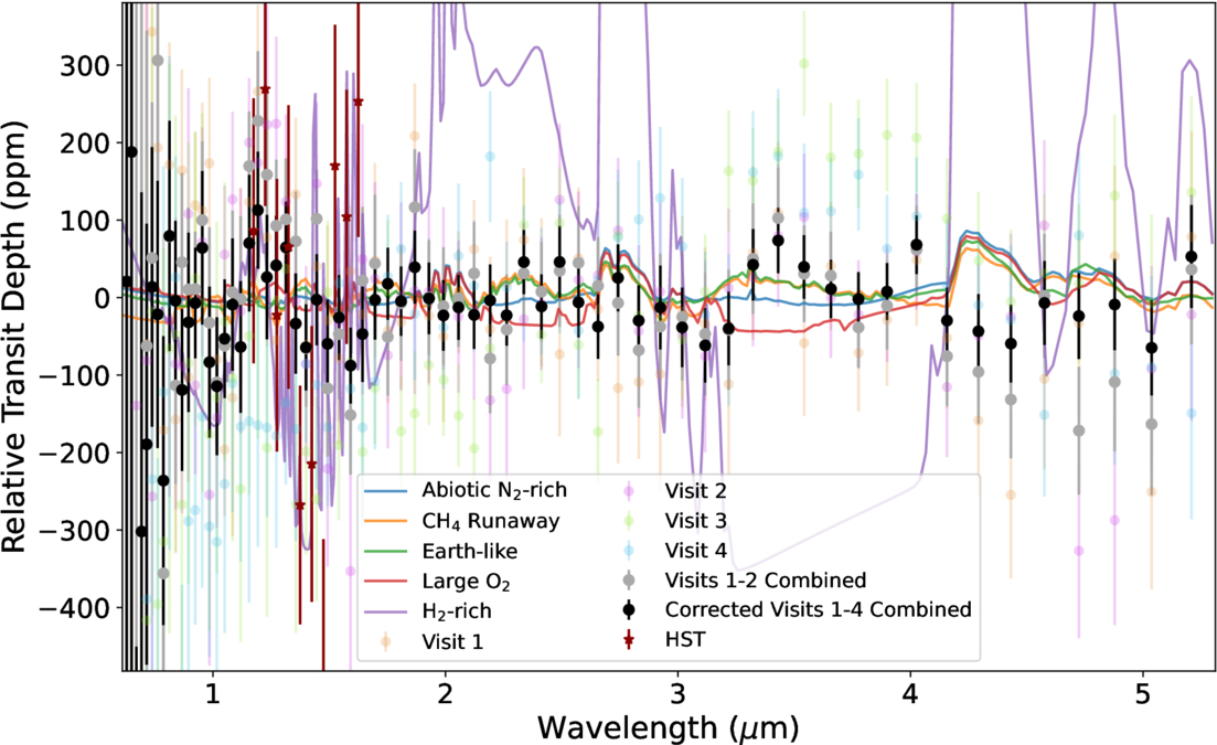
JWST spectra of TRAPPIST-1e (circles) and model outputs for several different atmospheric compositions and pressures (lines). Click to enlarge. [Glidden et al. 2025]

Ana Glidden (Massachusetts Institute of Technology) and collaborators used JWST to collect transmission spectra of the exoplanet TRAPPIST-1e. The team found evidence of stellar contamination in all of their observations, and they found that the data didn’t lean strongly in favor or against the planet having an atmosphere. Venus-like or Mars-like atmospheres were disfavored, hydrogen-rich atmospheres with traces of methane and carbon dioxide were excluded, and nitrogen-rich atmospheres with traces of methane and carbon dioxide were permitted.

Why it’s interesting:

TRAPPIST-1e is one of seven confirmed planets orbiting TRAPPIST-1, a cool M-dwarf star that is just larger than Jupiter and only 41 light-years away. All of these planets are roughly the size and mass of Earth, and as many as four of them — planets d through h — are thought to lie within the tiny star’s habitable zone. Thus, this system offers an excellent opportunity for powerful observatories like JWST to characterize the atmospheres of several potentially habitable planets. This study by Glidden’s team presents JWST’s first look at TRAPPIST-1e’s atmosphere through transmission spectroscopy.

How TRAPPIST-1 complicated the observations:

When examining an exoplanet that closely orbits its host star, special care must be taken to separate the signals from the planet and the star. This is especially tricky for active stars like TRAPPIST-1, whose surfaces are peppered with dark starspots and bright faculae. TRAPPIST-1’s surface features have contaminated observations of other planets in the system, as described in previous research, and these observations of TRAPPIST-1e were not exempt from the star’s meddling. Luckily, researchers are conducting further JWST observations that should help disentangle the star’s impact; an ongoing program will capture closely spaced transits of TRAPPIST-1e and TRAPPIST-1b, which trace nearly the same track across the star’s disk. Since TRAPPIST-1b appears to be a bare rock, any features that are shared between its spectrum and TRAPPIST-1e’s are likely to come from the star. Identifying these features will allow for better characterization of TRAPPIST-1e’s spectrum and atmosphere.

Citation

Ana Glidden et al 2025 ApJL 990 L53. doi:10.3847/2041-8213/adf62e

The post Selections from 2025: JWST Searches for an Atmosphere on TRAPPIST-1e appeared first on AAS Nova.

Standing on a Sub-Neptune

5 November 2025 at 17:00

A rendering of a blue planet in the foreground and a small bright star in the background.

Astronomers often assume that sub-Neptune exoplanets have magma oceans hiding beneath their atmospheres. New research suggests that this might not always be the case.

Puzzling Type of Planet

In the 30 years since the discovery of the first exoplanet, astronomers have come to appreciate that many of the most common planets in our galaxy look nothing like the worlds in our solar system. One type of planet in particular appears to be ubiquitous despite not appearing in our own cosmic neighborhood: sub-Neptunes. As their name suggests these planets are slightly smaller than Neptune, but still much larger than Earth or what we’d expect from a planet composed mostly of rock.

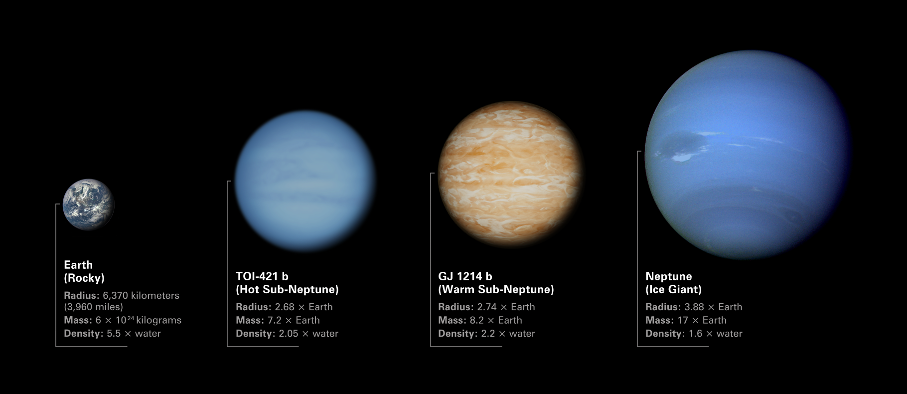
Four planets side by side ordered by increasing size. From left to right, they are Earth, TOI-421 b, GJ 1214 b, and Neptune.

An illustration of how two sub-Neptunes mentioned in this study (TOI-421b and GJ 1214b) compare with planets in our solar system. Click to enlarge. [NASA, ESA, CSA, Dani Player (STScI)]

What sub-Neptunes are made of and how they formed are still mysteries under active investigation by the research community. It is possible that these worlds are mostly rocky and sport puffy, light atmospheres over their surfaces; it’s also possible that these worlds are watery, and that most of their mass comes from heavy, steamy atmospheres. In most cases, though, it’s assumed that the high pressures and temperatures at the surfaces of these worlds foster a permanent, fiery magma ocean.

This key assumption that there’s no solid surface to stand on influences our models about how these planets cool and evolve over time. However, new research led by Bodie Breza (University of Maryland) suggests that this premise might not always be appropriate.

Solid Ground

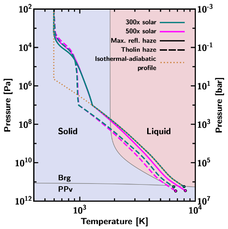
To test the assumption that every sub-Neptune has a magma ocean, Breza and collaborators simulated hundreds of thousands of feasible exoplanet interiors and atmospheres. Each simulation slightly tweaked various characteristics, like the surface temperature or the planet’s total mass, then checked whether the temperature and pressure conditions at the planet’s surface would leave any rocks in solid or liquid form.

phase diagram for a common rocky material

A phase diagram for a common rocky material MgSiO3. The various lines show different model pressure–temperature profiles for the sub-Neptune GJ 1214b, while the circles indicate the location of the atmosphere/surface boundary. All circles fall into the “solid” part of the phase diagram, indicating that GJ 1214b likely has a solid surface. [Breza et al. 2025]

Somewhat surprisingly, the team found that about a third of the models they simulated had solid, not magma, surfaces. They found there were two distinct ways to solidify the magma and create a firm shell. First and most intuitively, if the surface temperature falls low enough, the magma will simply freeze. Second and more intriguingly, they found that a planet can also suppress a magma ocean if its atmosphere is heavy enough to drive up the surface pressure beyond the solid–liquid threshold.

This latter result is particularly insightful in light of recent JWST observations that suggest many sub-Neptunes have heavy atmospheres. These new models suggest that these worlds might have solid surfaces, and that models attempting to explain their compositions should be tweaked to account for this finding. In these early days where astronomers are still puzzling out the most basic properties of these strange worlds, research like this demonstrates the power of using advanced theoretical modeling to help interpret our cutting-edge observations.

Citation

“Not All Sub-Neptune Exoplanets Have Magma Oceans,” Bodie Breza et al 2025 ApJL 993 L46. doi:10.3847/2041-8213/ae0c07

The post Standing on a Sub-Neptune appeared first on AAS Nova.

Planets Can Be Bells: The Aftermath of Major Mergers

24 October 2025 at 17:00

A rendering of two rocky worlds mid-collision, with debris exploding outwards.

What would happen to a gaseous exoplanet if it was struck by a protoplanet? Recent research suggests that it would ring like a bell, and that just maybe, we’d be able to observe this ringing back on Earth.

Heavy Metal Mystery

Previous studies have hinted that giant planets have more heavy elements in their cores than we’d expect if they had formed from the exact same stew of gas and dust as their host stars. How exactly they end up with these enriched compositions is something of a mystery, though. Astronomers have proposed two potential theories: one somewhat dull, and one that involves dramatic collisions between the massive protoplanets.

In the first case, perhaps growing giant planets clear out the gas along their orbits, then steadily and quietly accrete the dust that spills over into the gaps. In the latter case, theorists have conjured a model in which growing gas giant planets repeatedly collide and merge with large and somewhat rocky protoplanets. Both of these mechanisms would produce the enhanced heavy element contents observed today, so how can we tell these two paths apart? Recent work by a team led by J.J. Zanazzi (University of California, Berkeley) proposes one such test.

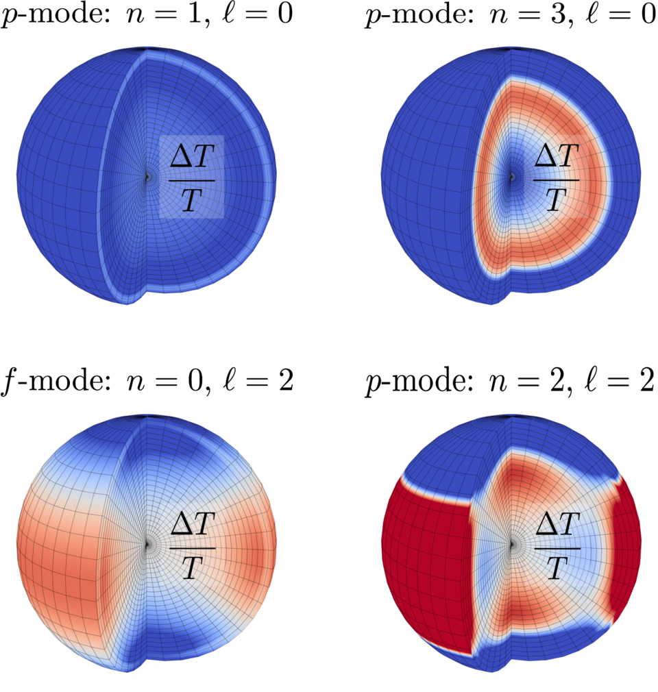
Four spheres each showing a different oscillation mode, colored red and blue according to the change in temperature.

An illustration of the different oscillation modes within a gas giant after it’s struck by a protoplanet. [Zanazzi et al. 2025]

Ringing Planets

Through mathematical derivations, the researchers demonstrate that if a gas giant were to collide with a protoplanet, the impact would cause the planet’s surface to physically oscillate inwards and outwards, and for its surface temperature to vary. In other words, the planet would “ring” like a bell struck with a hammer, and as it physically convulses in the aftermath of the merger it would grow brighter and fainter in a repeating, periodic pattern. In principle, if the ringing lasts for long enough and the oscillations in brightness were large enough, observers back on Earth could record the amplitude and period of the changes and back out some constraints on what had happened and when.

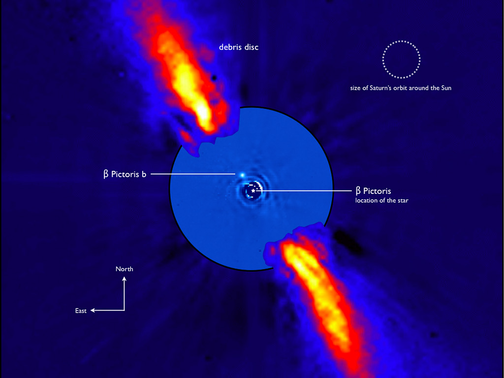
An image of a bright disk, edge on, a coronograph mask blocking out the star, and a bright dot near the center of the mask.

An image of Beta Pictoris, including the young gas giant Beta Pictoris b and the surrounding debris disk. Click to enlarge. [ESO/A.-M. Lagrange et al.; CC BY 4.0]

Excitingly, the researchers demonstrate that not only would the oscillations last for millions of years, they would also be bright enough for JWST to detect for one specific planet named Beta Pictoris b. Should this world have undergone a merger in the last 18 million years, just a few hours of observations with JWST’s Near-Infrared Camera would reveal 45-minute pulsations in which the planet’s brightness changes by about 1%. Since the planet is too far away from its host star for these oscillations to be caused by any gravitational interactions, detecting any periodic signal would be a slam-dunk for the major merger theory.

Beta Pictoris b is a young planet in a system that’s still forming, and it orbits its host star on an eccentric path that takes it through dense regions of the disk. Hopefully, future observations will test whether this treacherous path produced any massive collisions in the relatively recent past. Until then, though, we can all enjoy charming visions of massive planets colliding with one another and ringing through the night.

Citation

“Seismic Oscillations Excited by Giant Impacts in Directly Imaged Giant Planets,” J. J. Zanazzi et al 2025 ApJ 993 3. doi:10.3847/1538-4357/ae04ec

The post Planets Can Be Bells: The Aftermath of Major Mergers appeared first on AAS Nova.

Researchers Spot a Rare Glowing, Growing Planet

8 October 2025 at 17:00

WISPIT 2b

Have you ever eaten a meal so quickly that you started to glow? Although this behavior likely isn’t relatable for most humans, astronomers are beginning to find more and more baby planets doing just that.

Planetary Glow Up

Planets are, famously, quite large. But astronomers know that they don’t start out that way, and that instead, stars and planetary systems start as wispy collections of dust and gas. This raw material eventually compresses itself into stars and planets and life capable of contemplating such things, but how exactly that happens is not perfectly understood.

A colored-pencil drawing of gas flowing around a planet, with arrows noting the direction of the flow at various points.

A schematic of some of the processes involved during giant planet formation. Click to enlarge. [Batygin 2018]

Astronomers have the broad contours sketched out at least. Protoplanets destined to become gas giants like Jupiter and Saturn start by gobbling up all the material around them and eventually clear out gaps in the disks in which they are born. What little material flows into these gaps gets sucked onto the planet in a process called accretion, though exactly where this material lands and how gravity and magnetic fields interact is up for debate.

A number of different mechanisms predict that during this process, the protoplanet should emit light at a certain frequency associated with electrons jumping between energy levels in hydrogen atoms — what astronomers call Hα emission. In other words, they should glow at that specific wavelength only when they are accreting, though how strongly and consistently will depend on exactly what is happening around the planet.

These ideas existed only on paper until 2019, when a team first observed two glowing, growing planets around the star PDS 70. Recently, however, a powerful new instrument has begun collecting data, and astronomers just announced it has found another similar protoplanet: WISPIT-2b.

A New Discovery

A team of researchers led by Laird Close (University of Arizona) announced the discovery of this new world after analyzing images taken with the powerful new MagAO-X instrument on one of the 6.5-meter Magellan telescopes in Chile. The team outfitted the camera with a narrow filter that only admitted the Hα emission associated with accretion, then collected thousands of images over about two hours in April 2025. After stacking and post-processing their data, a faint dot jumped out beside the central star, right in the gap between two bright rings in the star’s disk.

A bright dot beside fainter rings of material.

A follow-up image of WISPIT-2b taken with a broader filter. [Laird et al. 2025]

This protoplanet, which the authors name WISPIT-2b in honor of their Wide Separation Planets in Time (WISPIT) survey, is likely about five times the mass of Jupiter and only 5 million years old, making it a baby on astronomical timescales. Based on how strongly it’s glowing, the team estimates that it’s accreting the equivalent of about 100 times the mass of Phobos, Mars’s largest moon, each year. This process won’t continue forever, as eventually the remains of the star’s disk will disperse and the planet will have to go hungry.

This remarkable find is only the third protoplanet unambiguously found to be embedded within a disk, and the first to be found in the gap between rings in a disk. With MagAO-X collecting data and the WISPIT survey underway, we’re likely in store for many other discoveries in the coming years. With enough observations and examples of these growing worlds, astronomers will fill in their models of how exactly giant planets as we know them are formed.

Citation

“Wide Separation Planets in Time (WISPIT): Discovery of a Gap Hα Protoplanet WISPIT 2b with MagAO-X,” Laird M. Close et al 2025 ApJL 990 L9. doi:10.3847/2041-8213/adf7a5

The post Researchers Spot a Rare Glowing, Growing Planet appeared first on AAS Nova.

Finding Avatar’s Pandora: Exomoons with Astrometry

6 October 2025 at 17:00

Illustration of a giant planet with a large moon orbiting a distant star

Editor’s Note: Astrobites is a graduate-student-run organization that digests astrophysical literature for undergraduate students. As part of the partnership between the AAS and astrobites, we occasionally repost astrobites content here at AAS Nova. We hope you enjoy this post from astrobites; the original can be viewed at astrobites.org.

Title: Astrometric Methods for Detecting Exomoons Orbiting Imaged Exoplanets: Prospects for Detecting Moons Orbiting a Giant Planet in α Centauri A’s Habitable Zone
Authors: Kevin Wagner et al.
First Author’s Institution: University of Arizona
Status: Published in ApJL

Six of the eight planets in our solar system host at least one moon; the innermost planets Mercury and Venus are the exceptions. The origins of these moons are widely studied and hotly debated. Earth’s very own moon seems to have formed in the aftermath of a collision between the young Earth and another protoplanet. Mars seems to have captured two asteroids as its moons, Phobos and Deimos, a process thought to have produced many of the irregular satellites orbiting the gas giants as well. Using our solar system as a model, the presence of moons seems like a natural outcome of planet formation.

Why then don’t we observe exomoons, moons orbiting any of the ~6,000 known exoplanets? Well, the largest moon in our solar system, Ganymede, is 2.5% as massive as Earth and has 40% of the radius, making it marginally larger than Mercury but still less massive. You might have heard how difficult it is to find Earth-like exoplanets, and finding exomoons is even harder. A few exomoon candidates have been announced via microlensing and transits, but the authors of today’s article investigate whether a different technique, astrometry, could help find moons.

Astrometry involves precisely tracking the positions of objects like stars or planets on the sky. In a simple star–planet system, the star and planet trace out ellipses around their shared center of mass. With a moon present, there is an additional deviation, as the planet wobbles to and fro due to the gravitational tug of the moon. The authors of today’s article check whether moons can be detected by tracking such wobbles exhibited by directly imaged planets.

To start, the authors consider whether any known planets are promising targets for astrometric moon searches. There just so happens to be a giant planet candidate in Alpha Centauri, and if there were a massive moon orbiting this large planet around this nearby star, it would be as good as it gets. The authors simulate orbits of this system (a Saturn-like planet in a 1.8 au orbit around a Sun-like star at a distance of 4.2 light-years) with a 30-Earth-mass moon injected. They simulate observing such a system with a space-based 6.5-meter telescope (similar to the planned Habitable Worlds Observatory) with realistic noise over a 3-year observing campaign. The simulated and modeled orbits are shown in Figure 1. After the authors subtract the best-fit planet orbit, they are left with what is shown in Figure 2, where a clear periodic perturbation from the moon as it orbits is visible.

plots of the hypothetical orbit of a moon in the Alpha Centauri system

Figure 1: Left: The zoomed-out orbit of the hypothetical Alpha Centauri star–planet–moon system. The blue curve shows the Keplerian orbital fit. Right: The zoomed-in orbit. The red points are the simulated observations, showing deviations caused by the moon. [Wagner et al. 2025]

plot showing deviations in position of the planet’s orbit over time

Figure 2: Left: Deviations in position of the planet’s orbit over time. The red points show the simulated observations, and the black curve shows the data smoothed. Right: Zoom-in showing the moon’s effect on the planet’s motion. [Adapted from Wagner et al. 2025]

The authors then repeat this procedure with more realistically sized moons and a more optimistic observing campaign (5-year baseline, 1-hour observing cadence, precision of 0.1 milliarcsecond) looking at the Alpha Centauri giant planet candidate. They use the difference in the chi-squared (χ2) test statistic to determine whether the presence of a moon is statistically preferred. Figure 3 shows the moon-induced deviations for two different moon masses and the resulting χ2 difference. Using their χ2 difference threshold of ~5, the lowest-mass detectable moon is ~0.2 Earth mass. This is much more massive than the Moon, which is around 1% of Earth’s mass. The authors additionally vary the moon’s orbital period and find that periods of 4–30 days are detectable.
plot of periodic position deviations caused by a moon

Figure 3: Left: Moon-induced planet position deviations over the first 90 observing days. Middle: Deviations from the entire 5-year observing baseline folded around the best-fit moon orbital period. Right: χ2 difference as a function of period, showing a peak in the signal at the moon’s orbital period. [Adapted from Wagner et al. 2025]

The authors continue to consider more specific observing scenarios: a 39-meter ground-based telescope (similar to the planned European Extremely Large Telescope) and a 3-meter space telescope built specifically to find moons. They find that the ground-based telescope observing once per day could detect an Earth-mass moon around a Saturn-like planet over a 5-year observing campaign. The dedicated space telescope observing once per hour could make the same detection observing over 5 years. While detecting moons astrometrically is neither easy nor fast, it may be feasible to start finding moons around planets orbiting nearby stars in the coming decades.

All of this is great news for fans of the hit movie (and still the highest-grossing movie of all time) Avatar, which features a habitable exomoon in the Alpha Centauri system. Searching for moons will help us understand their properties and formation, probe whether our solar system is unique, and even look for life on rocky moons orbiting gas giants in the habitable zones of their stars.

Original astrobite edited by Ryan White.

About the author, Kylee Carden:

I am a PhD student at Johns Hopkins University, where I am an observer of planets outside the solar system. I’m interested in dynamics, disks, demographics, the Roman Space Telescope. I am a huge fan of my cat Piccadilly, cycling, and visiting underappreciated tourist sites.

The post Finding Avatar’s Pandora: Exomoons with Astrometry appeared first on AAS Nova.

❌