For decades, astronomers have tried to decipher the source of carbon oxides on Uranus’s largest moons from ground-based telescopes. A recent study has leveraged JWST spectroscopy and laboratory experiments to identify carbon oxides and their origins for Ariel, Umbriel, Titania, and Oberon.

Unknown Origins of Carbon Oxide Enrichment

Forty years ago, the Voyager 2 spacecraft flew past Uranus and its twenty-seven moons, sending back prized portraits of the planet’s large and tidally locked satellites Miranda, Ariel, Umbriel, Titania, and Oberon. These images revealed extensive valleys, smooth plains, deep canyons, and possible icy volcanic (cryovolcanic) activity across the surfaces of the icy moons — the telltale signs of intense geologic activity. While Voyager 2 could take spectacular pictures, the spacecraft was not capable of identifying the molecules and materials making up these active surfaces.

Voyager 2 images of Uranus’s six largest moons. Click to enlarge. [NASA / JPL-Caltech / Ted Stryk; CC BY-NC-ND 4.0]

Ground-based detections are limited due to contamination from Earth’s atmosphere as well as the overall weakness of the carbon dioxide spectral features, thus space-based near-infrared observations of the Uranian moons are necessary to better constrain the carbon oxides on the satellites. Luckily, JWST’s Near-Infrared Spectrograph (NIRSpec) now offers astronomers unimpeded access the moons’ carbon oxide spectral features.

Chemical Clues from Space and in the Lab

In 2024, a study acquired NIRSpec observations of Uranus’s moon Ariel, revealing prominent carbon dioxide features and confirming the presence of carbon monoxide ice hinted at by ground-based studies. Expanding on these observations to include Umbriel, Titania, and Oberon alongside Ariel, Richard J. Cartwright (Johns Hopkins University) and collaborators obtained JWST NIRSpec spectroscopy of Uranus’s four largest moons in hopes of disentangling the origin story of their carbon oxides.

Diagram illustrating the leading and trailing sides of a moon orbiting Uranus. Click to enlarge. [AAS Nova/Kerry Hensley]

Spectral ratios of the trailing and leading hemispheres for each moon, labeling spectral features of multiple carbon-bearing molecules. Click to enlarge. [Cartwright et al 2026]

Carbon Oxide Origins

What does this mean for the origins of the carbon oxides on the Uranian moons? Spectral features of carbonate minerals and the widespread presence of carbon dioxide throughout the Uranus system suggest that these compounds exist natively. On the other hand, the concentration of carbon oxide features on the trailing hemispheres supports radiolytic production as these hemispheres are bombarded with more ionizing particles from Uranus’s magnetosphere.

Based on these results, the authors have postulated that both origin scenarios, native presence and radiolysis, are required to fully explain the presence of carbon oxides. Future laboratory studies and JWST observations will continue to reveal the nature and composition of bodies in the Uranus system, furthering our understanding of our solar system siblings.

Citation

“Tracing the Source of Carbon Oxides on the Large Moons of Uranus,” Richard J. Cartwright et al 2026 Planet. Sci. J. 7 199. doi:10.3847/PSJ/ae8818

The post Breaking the Ice: Origins of Carbon Oxides on Uranian Moons appeared first on AAS Nova.

Astronomers have been measuring comets for centuries. But in December of last year, researchers collected a unique set of comet observations: they recorded some of the highest-quality data of one of the weirdest known comets while it was far from the Sun.

Simultaneous Spectra and Images

A few months after the famous interstellar comet 3I/ATLAS rounded the Sun and began its journey back into the space between the stars, a group of astronomers led by Nathan Roth (NASA Goddard Space Flight Center) aimed JWST in the direction of its retreat to watch it fade away. Using a special observing mode that leveraged the Integral Field Unit (IFU) in JWST’s Near Infrared Spectrometer, these observations didn’t result in just a single image of the comet, but a full stack of images, each corresponding to a different wavelength of light.

Using the IFU allowed the observers to combine the best of both regular imaging, which reveals spatial structure, and standard spectroscopy, which reveals wavelength dependencies. As a result, they could make spatially resolved maps of how the emission from the comet’s fuzzy atmosphere of gas and dust, or coma, changed with distance from the comet’s icy nucleus and angle to the Sun. Since different molecules radiate at different wavelengths, these maps in turn reveal the composition and geometry of 3I/ATLAS’s coma.

Mapping the Coma

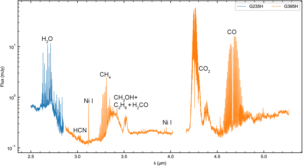
The spectrum of the coma of 3I/ATLAS. Note that this is a real spectrum, not a simulation. The contributions of various molecules are labeled alongside their most prominent emission lines. Click to enlarge. [Roth et al. 2026]

First, in contrast with normal solar system comets where water is the most abundant molecule, water was actually a secondary player here: there was significantly more carbon monoxide, or CO, than water in 3I/ATLAS’s coma. The researchers note that this might not be representative of the true distribution of the two species, but instead be the result of the timing of these observations. When observing a standard solar system comet, astronomers usually examine their targets when the object in question is within 2 au of the Sun. At these close distances, solar radiation is strong enough that water ice dominates the outgassing and activity in a coma.

However, these IFU measurements were taken when 3I/ATLAS was about 2.4 au from the Sun, or right in the transition region where water doesn’t sublimate as easily as CO or carbon dioxide (CO₂). It’s likely that as the comet approaches the so-called “ice line” where water will naturally freeze out, CO will only increase its domination of the coma.

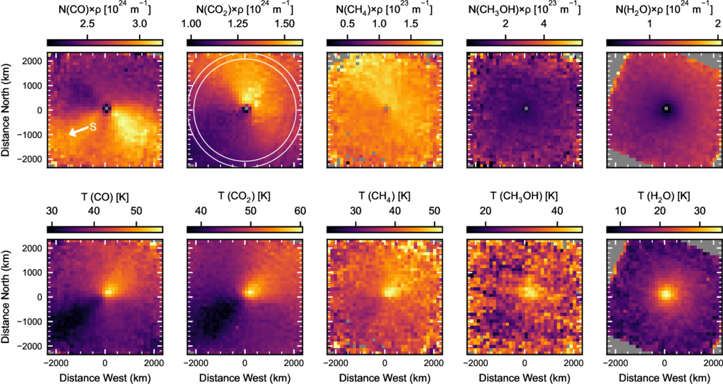
Top row: Maps of the distribution of various molecules in the coma. The white arrow shows the direction toward the Sun. Bottom row: The spatial distribution of the temperature of each species. Click to enlarge. [Roth et al. 2026]

Every Molecule for Itself

Second, each molecule seemed to be outgassing in its own unique direction from the coma. CO is leaving the nucleus in two different jets, one aimed directly back at the Sun and one perpendicular to it; CO₂ and methane (CH₄) are both leaking away in the anti-Sun direction; and water and methanol (CH₃OH) are sublimating in nearly spherically symmetric shells. The authors speculate that these geometries may be caused by different “active sites” on the comet, and that had they observed the comet for one full rotational period, they might have seen these jets pointing in different directions.

Although 3I/ATLAS is now too far and faint for observations like these, this study reveals just how much we can learn in the brief time interstellar visitors spend in our solar system. When the fourth interstellar comet inevitably wanders through the inner solar system, astronomers will doubtless be ready to use this observing mode again.

Citation

The post An Interstellar Comet’s Coma Composition appeared first on AAS Nova.

Exactly how the universe became reionized after cooling to form stars and galaxies remains an open question. A recent study investigates how a merging set of galaxies may have spurred an onslaught of ionizing photons into the intergalactic medium.

Lyman Continuum Leakers and Merging Galaxies

After its chaotic and blistering beginning, the universe cooled and began to coalesce, stars and galaxies flickering on to set the universe alight. From a few hundred million to about a billion years after the Big Bang, galaxies pumped high-energy ionizing Lyman continuum (LyC) photons into the intergalactic medium during what is known as the epoch of reionization. The exact mechanisms that produced and allowed LyC emission to escape galaxies during this era remain elusive.

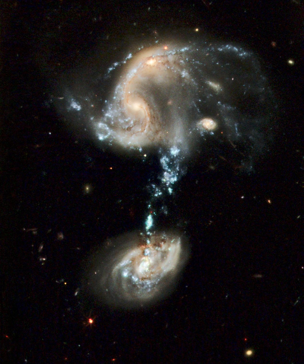
Hubble Space Telescope image of the interacting galaxy group Arp 194. The blue stream connecting the galaxies is where tidally stripped gas formed millions of new stars. [NASA, ESA, and the Hubble Heritage Team (STScI/AURA)]

While observational studies have increasingly pointed to galaxy mergers as considerable drivers of LyC escape, only a small number have explicitly considered the role of mergers in the epoch of reionization due to spectral and spatial resolution limitations. Leveraging the high-resolution capabilities of JWST, Shengzhe Wang (University of Chinese Academy of Sciences; National Astronomical Observatories, Chinese Academy of Sciences) and collaborators performed detailed analyses of two LyC-leaker candidates to better understand the role of galaxy mergers in heating up the universe.

Confirming (and Refuting) Merger-Driven Leaks with JWST

Using candidate LyC leakers first identified in the LymAn Continuum Escape Survey (LACES) carried out with the Hubble Space Telescope, Wang and team obtained high-resolution JWST spectroscopy for two galaxies at redshift z = 3.1 (about 2 billion years after the Big Bang), LACES94460 and LACES104037. After carefully identifying and measuring emission lines in each candidate, the authors confirmed LACES104037 as a merger-driven LyC leaker. However, the apparent LyC emission from LACES94460 was determined to be contamination from a low-redshift object.

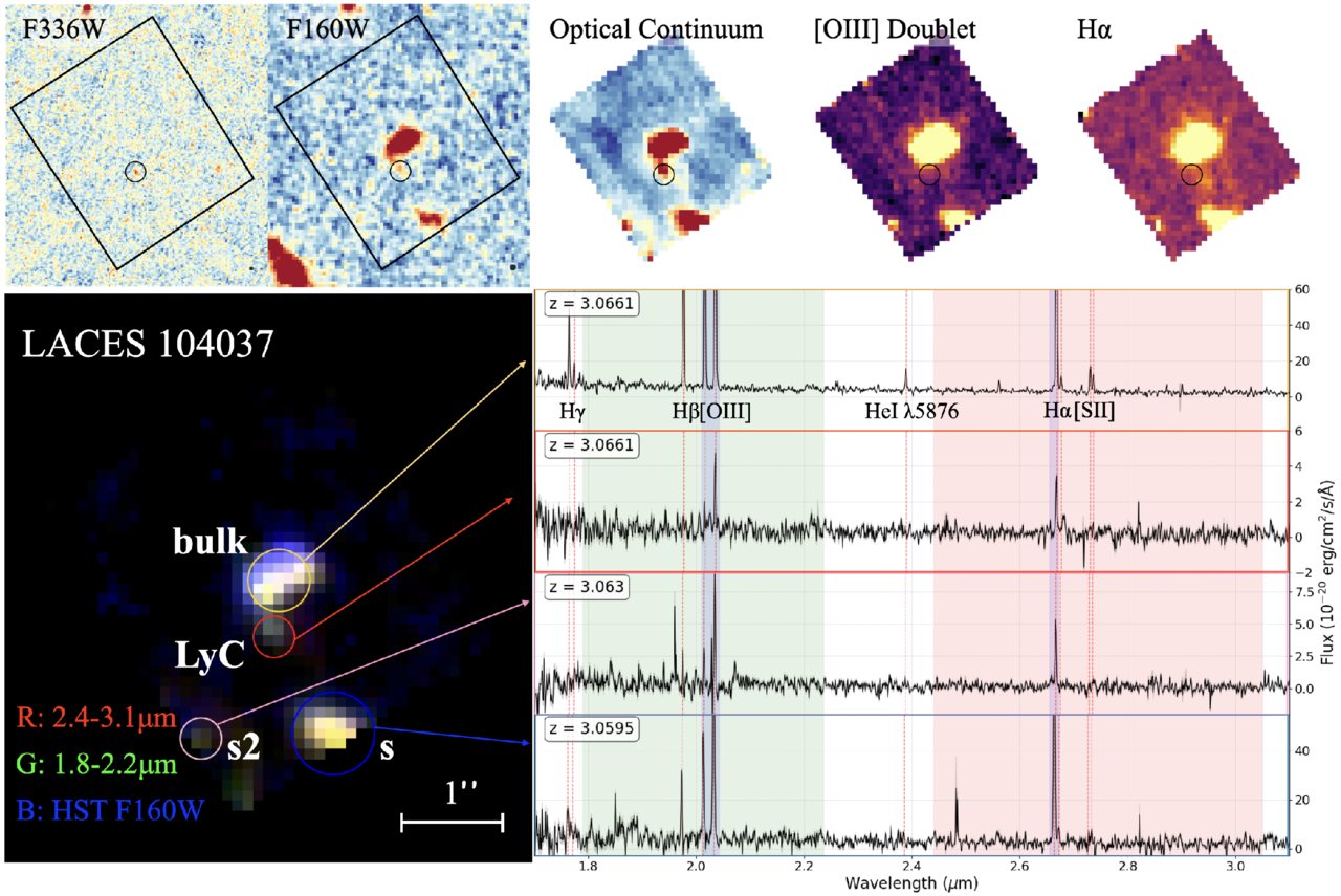
Hubble and JWST observations of LACES104037. The top panels show the Hubble images (first two panels) and the JWST spectral observations (last three panels). The bottom panel shows a composite three-color image marking the location of two primary interacting galaxies and the LyC emission along with the associated spectra. Click to enlarge. [Wang et al 2026]

LACES104037-LyC represents the first confirmed LyC leaker of its kind: an external clump of star formation in a tidal tail. This discovery aids in our understanding of how mergers can drive high-energy photon emission, and highlights the critical role galaxy mergers may play in the epoch of reionization. Future high-resolution observations will hopefully reveal more knots of LyC-leaking stars within merging galaxies and provide a deeper understanding of this important evolutionary phase of the universe.

Citation

“Confirmation and Refutation of Lyman Continuum Leakers at z ~ 3 with JWST NIRSpec IFU,” Shengzhe Wang et al 2026 ApJL 1006 L17. doi:10.3847/2041-8213/ae8523

The post A Lyman-Leaking Galaxy Merger Confirmed with JWST appeared first on AAS Nova.

Ultra-hot Jupiter WASP-121b is once again puzzling astronomers. New JWST observations have revealed aspects of this superheated planet’s atmosphere that models cannot yet explain.

An Extreme Planet

Among the more than 6,000 known exoplanets, there are many types of worlds that aren’t represented in our solar system. The most exotic and unfamiliar planets might be the ultra-hot Jupiters: giant planets nestled so close to their host stars that they are tidally locked, with temperatures on their permanently starlit sides climbing to thousands of degrees.

WASP-121b, which circles its F-dwarf host star every 30.5 hours, is one of the best-studied ultra-hot Jupiters. Previous work has started to reveal the complexity of its atmosphere, and now, data from JWST have opened a new window onto WASP-121b’s behavior.

New View from JWST

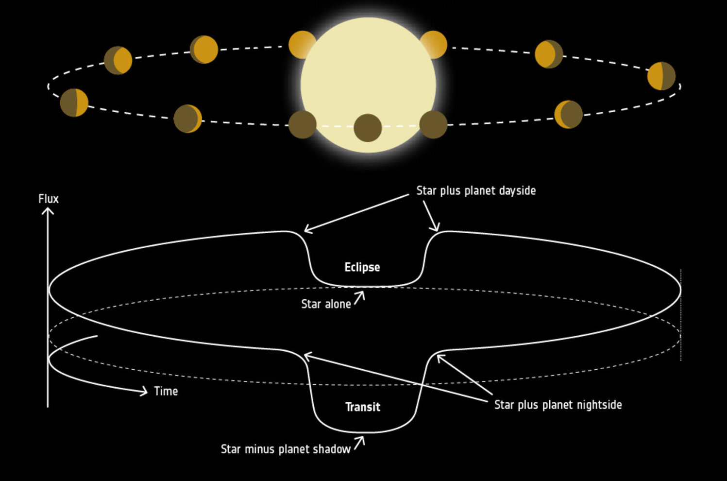
A representation of an exoplanet’s phase curve. Click to enlarge. [ESA]

The team used two 3D general circulation models to predict the planet’s atmospheric structure and extract synthetic spectra and phase curves to compare against the JWST observations. Using nine model configurations in total, the team varied several inputs, including sources of atmospheric opacity, sources of atmospheric drag, and assumptions about whether clouds are able to form on the planet’s cooler nightside.

Left with a Mystery

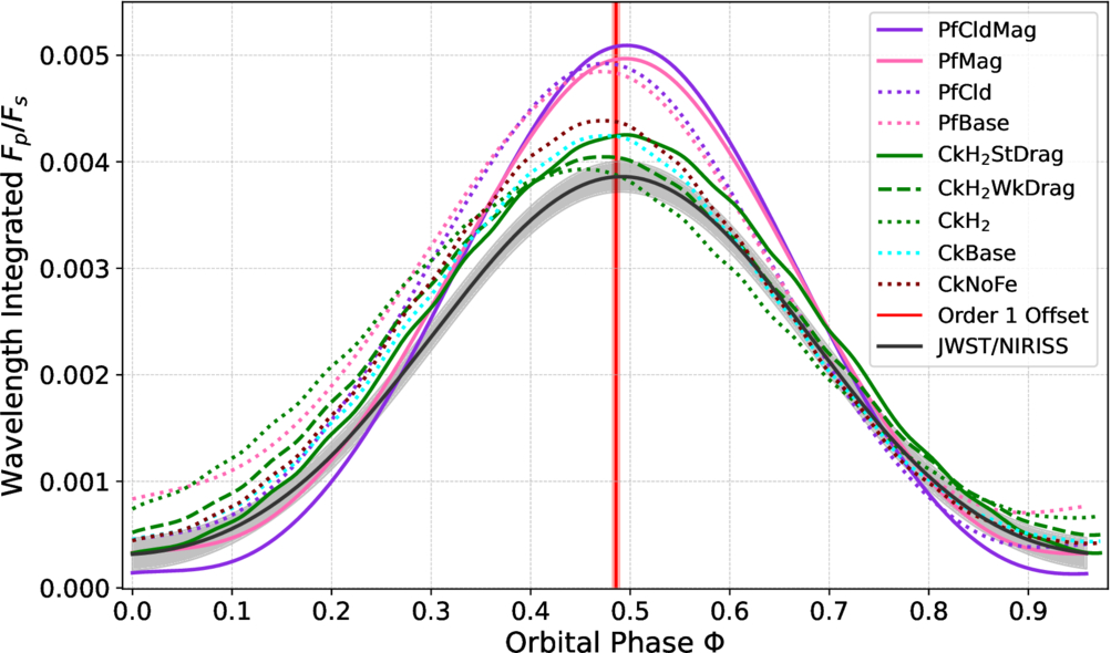
Frazier and collaborators found two aspects of WASP-121b’s phase curve that their models couldn’t explain: the planet emits less light overall than predicted, and the location of its phase-curve offset changes with wavelength.

Modeled phase curves, shown as the flux of the planet divided by the flux of the star, for WASP-121b (colored solid and dotted lines) compared to the best fit to the JWST observations (black line). Click to enlarge. [Frazier et al. 2026]

The phase-curve offset is the difference between a planet’s sub-stellar point (where the star is directly overhead) and the brightest point in the planet’s atmosphere. In general, some degree of offset is expected because planetary winds tend to whisk heat away from the sub-stellar point, placing the brightest point somewhere to the east (usually). For WASP-121b, the offset is unexpectedly small — suggesting a source of drag in the atmosphere that prevents winds from transporting heat away from the sub-stellar point — and it’s larger at shorter wavelengths. This wavelength dependence isn’t predicted by any of the models, and it’s not clear what causes it.

These results demonstrate something remarkable: that our observations of a planet nearly 900 light-years away have become so precise that they’re pushing our already complex models to include more physics — an exceptionally exciting motivation for model improvement!

Citation

“The Days Drag On on WASP-121 b: Interpreting Its NIRISS Spectroscopic Phase Curve with General Circulation Models,” Robert C. Frazier et al 2026 ApJ 1004 102. doi:10.3847/1538-4357/ae69ca

The post Complexities and Mysteries in the Atmosphere of Ultra-Hot Jupiter WASP-121b appeared first on AAS Nova.

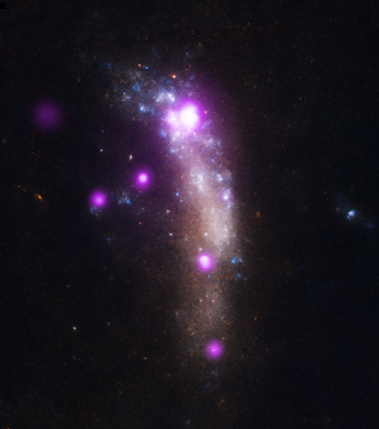
In 2010, the supernova SN 2010jl illuminated a corner of a small, irregular galaxy 150 million light-years away. More than a decade later, researchers have found evidence that this collapsing massive star has created a significant amount of cosmic dust.

Superluminous Supernova

This X-ray and optical image shows SN 2010jl in its host galaxy. The supernova is the brightest X-ray source, near the top of the galaxy. [X-ray: NASA/CXC/Royal Military College of Canada/P.Chandra et al); Optical: NASA/STScI]

SN 2010jl offers an excellent chance to study the dust-forming potential of core-collapse supernovae. This supernova was unusually luminous because of intense interactions between the expanding supernova shock and the dense material surrounding the exploding star, and it’s possible that these types of interactions spur the creation of dust. In the first few years after the supernova was discovered, researchers found evidence that it had produced new dust. What has it been up to since?

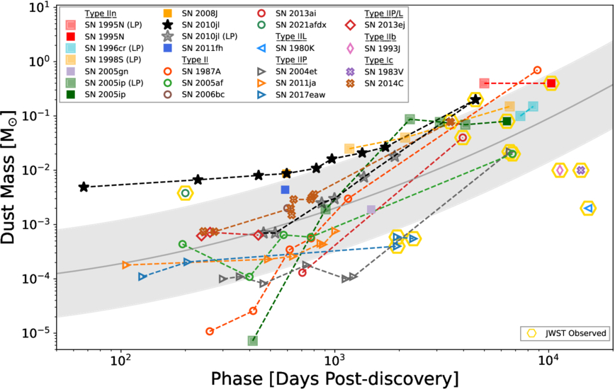
SN 2010jl’s inferred dust mass over time (black stars) compared to other supernovae. Click to enlarge. [Smith et al. 2026]

Checking Back In

Thirteen years after SN 2010jl was discovered, Nathan Smith (Steward Observatory) and collaborators checked in on its dust production. The team collected new ground-based optical spectra from the Keck I telescope and the MMT Observatory and mid-infrared spectra from JWST. The optical spectra — among the latest collected for any superluminous supernova — show numerous narrow emission lines that indicate that the expanding supernova continues to interact with its surroundings.

In the JWST observations, SN 2010jl is the brightest mid-infrared point source in its host galaxy. Through spectral energy distribution modeling, Smith and coauthors found that the brilliant infrared emission is likely due to a shroud of warm dust totaling roughly 20% of the mass of the Sun. This is about 80 times more dust than inferred from observations made a decade earlier.

Where’s the Dust?

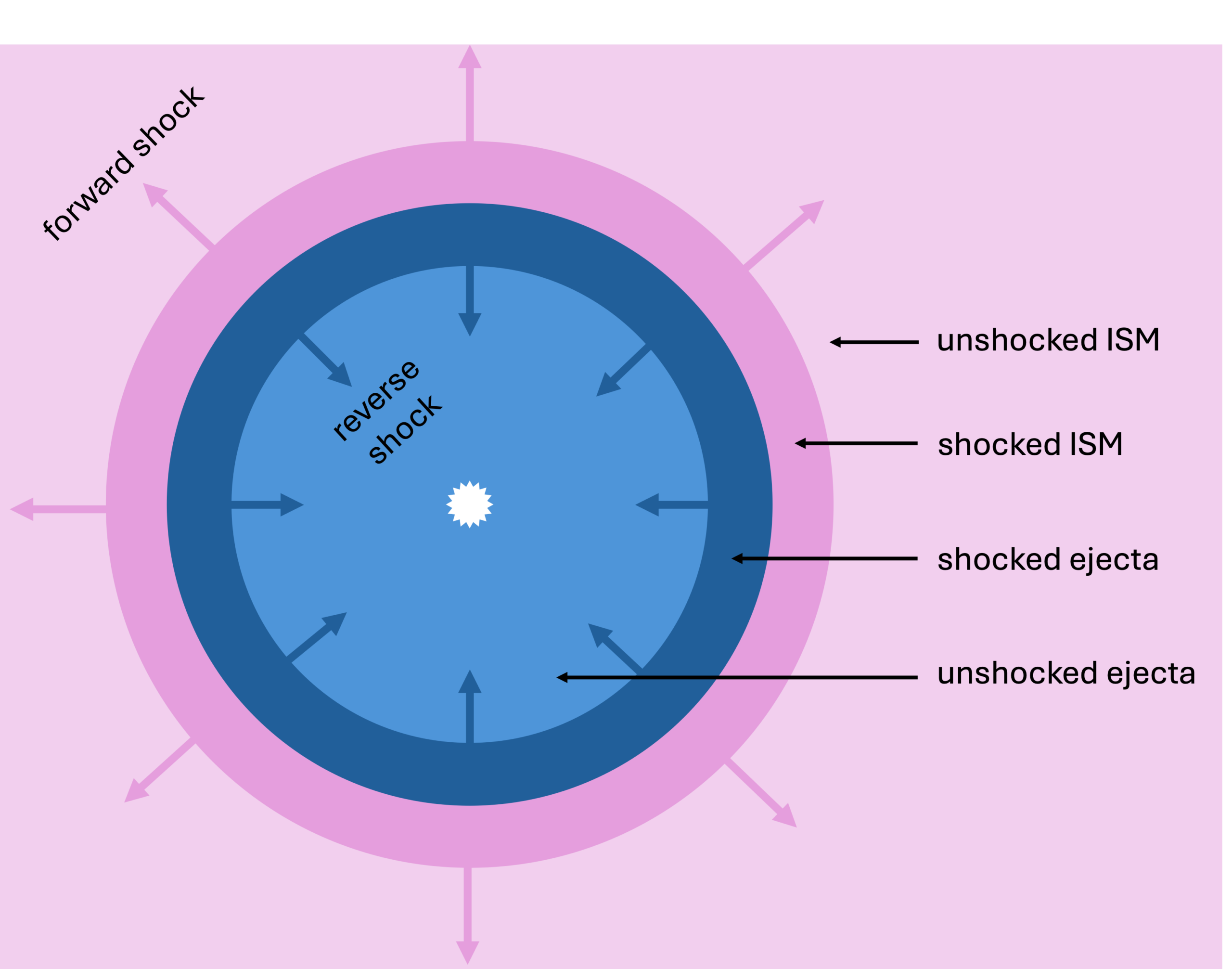
Diagram showing the outward-moving forward shock and inward-moving reverse shock of a supernova that is interacting with the interstellar medium (ISM). The post-shock region is located between the two shocks and contains shocked ejecta as well as shocked interstellar material. Click to enlarge. [AAS Nova/Kerry Hensley]

While it’s not possible to rule out the other options entirely, Smith and collaborators argue that at least some of the dust can be traced to new growth in the post-shock region. Because post-shock dust grains are likely to reach the interstellar medium, this suggests that superluminous, strongly interacting supernovae like SN 2010jl are a viable source of dust in the present-day universe and in high-redshift galaxies alike.

Citation

“JWST Spectra Indicate a Large Mass of Postshock Dust Formed by SN 2010jl,” Nathan Smith et al 2026 ApJ 1006 224. doi:10.3847/1538-4357/ae74c5

The post A Seriously Dusty Supernova appeared first on AAS Nova.

Editor’s Note: Astrobites is a graduate-student-run organization that digests astrophysical literature for undergraduate students. As part of the partnership between the AAS and astrobites, we occasionally repost astrobites content here at AAS Nova. We hope you enjoy this post from astrobites; the original can be viewed at astrobites.org.

Title: The JWST EXCELS Survey: Insights into the Nature of Quenching at Cosmic Noon
Authors: Maya Skarbinski et al.
First Author’s Institution: Johns Hopkins University
Status: Published in ApJ

How to Quench a Galaxy

Look at an image of the sky taken with a sufficiently sensitive telescope, and you’ll quickly notice that galaxies tend to cluster into two main types: blue spiral galaxies, which have flat disk shapes with a central bulge, and red elliptical galaxies, which look like spherical or elliptical balls of red stars. Blue spiral galaxies can form tens to hundreds of stars every year, while elliptical galaxies have completely stopped forming stars, meaning that some process has to transform star-forming spirals into non-star-forming, or “quiescent,” elliptical galaxies. To form the current population of massive elliptical galaxies, this process had to be common about 2–3 billion years after the Big Bang at “cosmic noon,” the period when star formation in the universe peaked. The processes that “quench” star formation in massive galaxies are still being studied, and one of the best ways to study them is to find galaxies that recently quenched and look for clues about the processes that quenched them.

Post-starburst galaxies are galaxies that have rapidly quenched after a short burst of star formation. Because these galaxies quenched so quickly and so recently, it’s often possible to find signs of whatever quenched them, like the signatures of past galaxy mergers, feedback from supermassive black hole accretion, or the shutoff of gas flowing into the galaxy. Rapid quenching is pretty uncommon now, but it was a much more common way for galaxies to quench at cosmic noon. Understanding post-starburst galaxies at cosmic noon is therefore critical for understanding the formation of massive elliptical galaxies in the local universe.

The Quest for Quenched Galaxies

Today’s article uses data from the JWST Early eXtragalactic Continuum and Emission Line Survey (EXCELS) to identify post-starburst galaxies at cosmic noon and try to determine why they quenched. EXCELS is a spectroscopic survey, so the authors get a spectrum for every galaxy. The spectrum encodes information about the galaxy’s stellar population, including the mass of stars in the galaxy, the number of stars forming every year, and the history of star formation throughout the galaxy’s life.

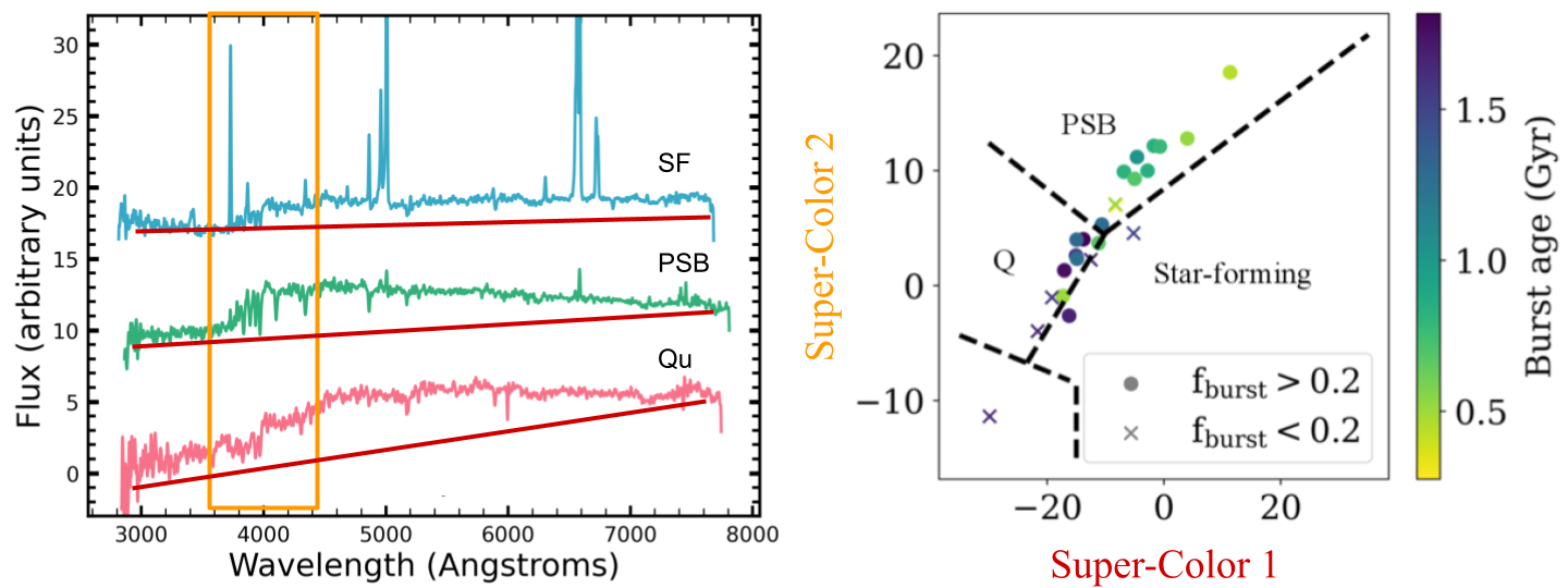
The authors use a technique called principal component analysis to further divide the sample into young and old post-starbursts. Principal component analysis is a machine-learning technique that learns the most important features of a data set. This technique is used for “dimension reduction,” or reducing the number of data points needed to learn something about the object. A typical spectrum has hundreds or even thousands of data points, which means performing data analysis on a spectrum can be very computationally expensive. Principal component analysis takes these thousands of data points and learns broad patterns that correlate with each other. These patterns are called “supercolors” in the context of spectral data, and they encode things like the overall shape and color of the spectrum as well as the spectral shape around key features (see Figure 1 for a visualization). Since the overall shape, color, and emission/absorption line features of a spectrum come from the galaxy’s stellar population, this method can be used to identify galaxies with lots of star formation a billion years ago but very little star formation today — in other words, post-starburst galaxies.

Figure 1: An example of principal component analysis for sample star-forming (SF), quiescent (Qu), and post-starburst (PSB) galaxy spectra (left-hand side). Principal component analysis simplifies a many-dimensional data set (for example, spectra) into fewer dimensions. In this case, Super-Color 1 measures the overall color of the spectrum (shown on the left-hand side as the slope of the spectra, marked with red lines), while Super-Color 2 measures the shape of the spectrum around 4,000 angstroms (orange box). The authors use principal component analysis to identify post-starburst galaxies for further analysis (right-hand side). [Adapted from Skarbinski et al. 2026]

The authors apply principal component analysis to the galaxies in their sample and find that 11 of the galaxies in their sample are classified as post-starburst, 9 are quiescent, and 4 still have some star formation. To further analyze the stellar populations of the post-starbursts in their sample, the authors use a program called Bagpipes to fit the galaxies’ spectra. Bagpipes is a spectral energy distribution fitting software, which means that it takes the observed spectrum of a real galaxy and tries to match it to a library of different stellar spectra. By measuring the relative contribution of different kinds of stars (which all have different lifetimes), Bagpipes can compute the likely history of star formation in the galaxy (e.g., when the star formation rate peaked) as well as the present-day properties of the galaxy (things like the mass in stars versus dust and the current star formation rate). The authors use the galaxies’ star formation histories to try to find clues as to how they quenched.

How Quickly Do Post-Starbursts Quench?

First, the authors measure something called a “quenching timescale,” which they define as the length of time between when the galaxy’s star formation rate peaked and when it fell low enough that the galaxy was quenched. The quenching timescale depends on which process shut down star formation in the galaxy — feedback from black hole accretion or star formation should cause fast quenching, while galaxies that are starved of gas from the intergalactic medium should quench more slowly. The authors find that 15 of their galaxies quenched in under 500 million years, 6 took between 500 million and 1 billion years, and 3 took longer than 1 billion years to quench. The galaxies that had the highest peak star formation rates quenched the fastest, suggesting that feedback from star formation could have played a role in quenching these galaxies.

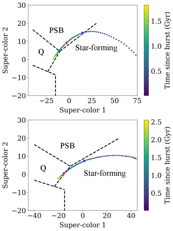
Figure 2: Possible evolutionary tracks in supercolor for two example galaxies as they quench. The galaxy in the top panel quenches quickly and has post-starburst supercolors for about a billion years, while the galaxy in the bottom panel quenches without ever going through the post-starburst phase. The authors use these tracks to determine how important the post-starburst phase is for quenching massive galaxies. [Skarbinski et al. 2026]

Next, the authors measure how important the post-starburst phase is to form massive quiescent galaxies. Not all galaxies that quench go through a post-starburst phase; some objects, especially those that quench slowly, will transition directly from star forming to quiescent. The authors use the star formation histories from their spectral energy distribution fits to predict how the galaxies’ supercolors changed after their star formation peaked (Figure 2) and find that six of the nine quiescent galaxies went through a post-starburst phase in the past, while the other three did not. For the objects that went through a post-starburst phase, the median time spent as a post-starburst was around 600 million years.The authors can use this measured “visibility timescale” to constrain whether the post-starburst phase is important for forming massive quiescent galaxies. If the fraction of post-starburst galaxies in a sample is high, that can be for two reasons: either a larger fraction of galaxies will eventually go through a post-starburst phase, or the post-starburst phase is very long, making it easy to find post-starburst galaxies. Using the measured timescale of 600 million years and combining with results from another article, the authors find that 40% of quiescent galaxies likely went through a post-starburst phase; for the more massive end of the sample, this fraction increases to around 73% due to the shorter visibility timescale. This suggests that the post-starburst phase is very important for forming the kind of massive quiescent galaxies we see in the local universe.

While the post-starburst phase is important, the different quenching timescales present across the sample suggest that multiple pathways existed to quench galaxies at cosmic noon, similar to what has been found in less-distant galaxies and at cosmic noon in other samples. This is also supported by the fact that four of the five galaxies with sufficient data show evidence of an actively accreting supermassive black hole that may help shut down star formation in many (but perhaps not all) massive galaxies. While the precise processes that quench massive galaxies are still uncertain, one thing is clear: JWST EXCELS at solving the mystery!

Original astrobite edited by Anavi Uppal.

About the author, Margaret Verrico:

I am a fourth-year graduate student at the University of Illinois Urbana-Champaign. I study the connection between supermassive black hole transients and their host galaxies. I am also an avid knitter and reader, and I am passionate about opening up STEM opportunities for people of all backgrounds.

The post EXCELlent Work, Detectives! Solving the Murder of Star Formation in Galaxies with JWST appeared first on AAS Nova.

The Bullet Cluster is best known for being considered a “smoking gun” for the existence of dark matter, but even a famous galaxy cluster like this one has its secrets. For more than two decades, different measurements of the merging clusters’ dynamical mass ratio have yielded vastly different results. In a recent research article, Boseong Young Cho (Yonsei University) and collaborators used data from JWST and the Dark Energy Camera to revisit the Bullet Cluster and measure its mass ratio using new data. The image above shows a near-infrared view of the Bullet Cluster from JWST, with an overlay of mass contours derived from gravitational-lensing measurements. The team’s analysis assigned a mass of 1.5 quadrillion solar masses for the main cluster (on the left side of the image above), and a mass of 150 trillion solar masses for the subcluster. This suggests a mass ratio of roughly 10, which matches the value supported by hydrodynamical simulations and cements the event as a minor merger. The team also identified three distinct cluster halos (two in the main cluster and one in the subcluster), providing an important constraint on the cluster configuration for future modeling. To learn more about this investigation of the Bullet Cluster, be sure to check out the full research article linked below!

Citation

“Joint JWST–DECam Lensing Reveals that the Bullet Cluster Is a Minor Merger,” Boseong Young Cho et al 2026 ApJ 1005 28. doi:10.3847/1538-4357/ae6a90

The post Featured Image: A Mass Mystery in the Bullet Cluster appeared first on AAS Nova.

Fullerenes — a class of molecules composed entirely of interconnected carbon atoms — are the largest molecules definitively detected in space. Researchers using JWST to study a planetary nebula have found new spectral features from a fullerene composed of 60 carbon atoms, offering another way to study how these molecules form and survive in space.

Full of Fullerenes

Planetary nebula Tc 1 as seen by JWST. [NASA / ESA / CSA / Western University, J. Cami]

Since that discovery, Tc 1 has been a hot spot for studies of buckyballs. However, researchers are still puzzling over how these large molecules form and survive in harsh space environments.

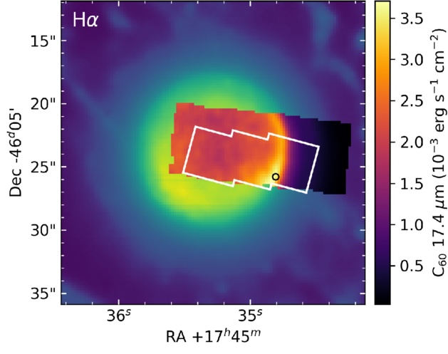
A closeup of the center of Tc 1, showing the region observed with JWST’s Mid-Infrared Instrument (black-to-yellow color scale) and Near-Infrared Spectrograph (white outline). The background color scale shows the nebula’s H-alpha emission as seen by the Very Large Telescope. [Adapted from Giese et al. 2026]

From Spitzer to JWST

Morgan Giese (The University of Western Ontario) and collaborators recently reported on the results of a JWST observing program that aimed to understand how fullerenes respond to changes in their environment. The team mapped the distribution of C₆₀ molecules at varying distances from the powerful ionizing radiation of Tc 1’s central star.

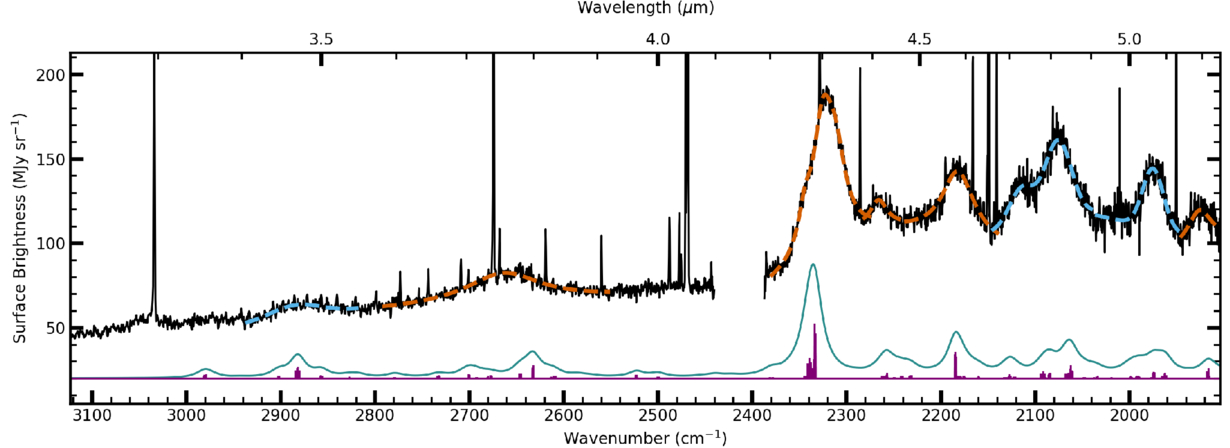
The team successfully spotted the emission features from the fullerene C₆₀ seen in earlier observations, but they also turned up something unexpected: a handful of prominent emission features from 3.5 to 5.2 microns that had not been reported previously.

Feature Presentation

What’s the source of these emission features? The distribution of the emission provides a strong clue: known spectral features from fullerenes C₆₀ and C₇₀ are concentrated in a narrow, bright ring around the center of the nebula, with diffuse emission suffusing the rest of the nebula — and the newfound spectral features follow the same distribution.

JWST spectrum of Tc 1 (black line) extracted from the area indicated by a black circle in the previous image. The orange and blue dashed lines show fits to the newfound emission bands, and the results of the anharmonic calculations are shown as the teal line below the JWST spectrum. Click to enlarge. [Giese et al. 2026]

Giese and coauthors found that 17% of the energy emitted by the C₆₀ molecules in Tc 1 is released in these  combination bands, suggesting that these features must be taken into account when modeling the cooling of C₆₀ molecules. The discovery of new fullerene spectral features also has implications for future studies of these molecules: since these features appear in a wavelength range where features from other complex molecules like polycyclic aromatic hydrocarbons are weak, these newly identified bands provide a promising way to spot and study fullerenes across space environments.

Citation

“Detection of C₆₀ Combination Bands in the Near-IR Spectrum of Tc 1,” Morgan M. Giese et al 2026 ApJL 1004 L32. doi:10.3847/2041-8213/ae76d5

The post New Spectral Signs of Buckyballs Discovered in Planetary Nebula appeared first on AAS Nova.

For the first time, astronomers have distinguished between the morning and evening atmospheres of a single planet, revealing two remarkably different environments at its edges. WASP-121 b is a gas giant that orbits extremely close to its star, resulting in one hemisphere exposed to temperatures approaching 2,500 degrees Celsius while the opposite side remains in constant darkness.

A research team from the Max Planck Institute for Astronomy used the James Webb Space Telescope to provide observational evidence for a phenomenon that models had previously predicted. The boundary regions between day and night on tidally locked planets can exhibit distinct temperatures and chemical compositions.

The recent findings appeared in a study published in Nature Astronomy.

A World Stuck in Time

WASP-121 b is part of a group of gas giants known as hot Jupiters. These massive planets orbit their stars in just a few days and eventually become locked in place by gravity. Tidal forces keep one side facing the star at all times, while the other side never sees daylight.

“WASP-121 b is particularly extreme,” said co-author Tom Evans-Soma of the University of Newcastle, Australia. “Average temperatures on the dayside hemisphere are around 2,770 Kelvin, while those on the nightside are closer to about 1,000 Kelvin.”

The difference in temperature between the two hemispheres, which is about 1,775 degrees Celsius, makes WASP-121 b one of the most thermally extreme exoplanets known. The regions at the boundary between day and night, called terminators, are where the planet experiences constant morning or evening conditions. Scientists expected these areas to have different atmospheric properties, but only with the precision of JWST could these differences be directly observed.

Mapping the Atmosphere

The researchers used a method based on the planet’s transit across its star to study these differences. As WASP-121 b passes in front of its star, it rotates by about 30 degrees, which means that different parts of its atmosphere can be observed during each transit. By tracking how infrared starlight filters through the atmosphere over time, the team reconstructed how temperature and chemical composition change across different longitudes.

“By measuring how starlight absorption changes as WASP-121 b rotates, we probe its atmosphere longitude by longitude,” said lead author Cyril Gapp of MPIA. The observations not only confirmed what models had predicted, but also showed that the differences between the two terminators are even greater than expected.

Two Different Skies

The evening side of the planet’s terminator absorbs more starlight than the morning side. Powerful eastward winds sweep heat from the scorching dayside toward the nightside, with the evening region getting the first blast of this warmth. This extra heat causes the atmosphere there to puff up, allowing it to absorb even more starlight, as the observations showed.

Chemical measurements backed up these findings. Carbon monoxide absorption increased as the hotter regions of the evening came into view near the end of the transit. Water showed a different pattern. Rather than simply decreasing with higher temperatures, the researchers interpret the result as evidence that water molecules in the upper atmosphere are breaking apart, likely due to the intense heat at the evening terminator. This points to a real chemical change, not just a shift in molecular location.

The Cloud Problem

The morning side shows a different environment. Although models predicted a difference between the two terminators, they did not fully explain why the morning side appears cooler and more opaque. The most likely explanation involves clouds that are unlike those on Earth.

At the morning terminator, air comes in from the cold nightside. Temperatures may be low enough for silicate and mineral compounds to turn into tiny particles, forming clouds that block infrared radiation from below. This makes the atmosphere appear cooler than it really is underneath.

When the team adjusted their models to account for these clouds, the results more closely aligned with their observations. Still, confirming exactly how these clouds form and behave will require more advanced modeling, as cloud formation and evaporation in such extreme environments remain a major puzzle in exoplanet science.

A Method Ready to Scale

WASP-121 b has been the subject of previous studies, but JWST now enables astronomers to examine its atmosphere in detail, section by section. This approach is now also available for use with other exoplanets.

The team has already found other ultra-hot gas giants with the right temperatures and orbits for similar analysis. Using this method on other planets will help astronomers compare atmospheric conditions and deepen our understanding of extreme planetary environments.

Austin Burgess is a writer and researcher with a background in sales, marketing, and data analytics. He holds an MBA, a Bachelor of Science in Business Administration, and a data analytics certification. His work focuses on breaking scientific developments, with an emphasis on emerging biology, cognitive neuroscience, and archaeological discoveries.

Editor’s Note: Astrobites is a graduate-student-run organization that digests astrophysical literature for undergraduate students. As part of the partnership between the AAS and astrobites, we occasionally repost astrobites content here at AAS Nova. We hope you enjoy this post from astrobites; the original can be viewed at astrobites.org.

Title: A Panchromatic JWST Spectrum of a Giant Starspot on the Fully Convective M Dwarf TOI-3884
Authors: C. A. Murray et al.
First Author’s Institution: University of Colorado Boulder
Status: Published in ApJ

We often picture stars as smooth, glowing spheres, as if they’ve been run through an Instagram filter. But real stars have spots: cooler, darker regions on a star’s surface caused by strong magnetic fields.

Annoyingly, these spots can seriously interfere with how we study exoplanet atmospheres.

How to Probe a Planetary Atmosphere

Planetary atmospheres are often probed through transmission spectroscopy. When a planet transits its star, some starlight passes through the planet’s atmosphere before reaching us. We can distinguish the light that has passed through the planet’s atmosphere by comparing the star’s light in transit versus out of transit. In doing so, we can isolate the atmospheric spectrum and look for absorption features of species like water or oxygen.

Easy, right?

How Starspots Get in the Way

Things get more complicated once we stop thinking of the star as if it’s been smoothed out by an Instagram filter. Starspots are cooler than the surrounding stellar surface, which means they emit a different spectrum. They are also constantly changing: new spots can form, old ones can disappear, and the star’s rotation carries them in and out of view. This changes things.

First of all, your star’s spectrum changes over time, which could mean that the star’s spectrum out of transit is not the same as the star’s spectrum during transit. On the other hand, the planet may transit across a starspot instead of a “normal” stellar region. In this case, the light we measure during the transit is affected by the spot, and it is no longer accurate to directly compare it with the overall stellar light outside the transit.

Ultimately, absorption features that we thought were from the planetary atmosphere could actually be coming from starspot contamination instead.

Starspot Models: Our Solution?

To deal with this, astronomers build starspot models, where they vary the spots in terms of the following:

• The surface covering fraction: this parameter tells us how much of the stellar surface is covered in spots
• The temperature contrast: this parameter tells us how much cooler (in ratio) the spot is compared to the rest of the stellar surface, and by proxy how much dimmer

These models are promising, but how do we know that we have chosen the right parameters?

A Unique Laboratory: TOI-3884

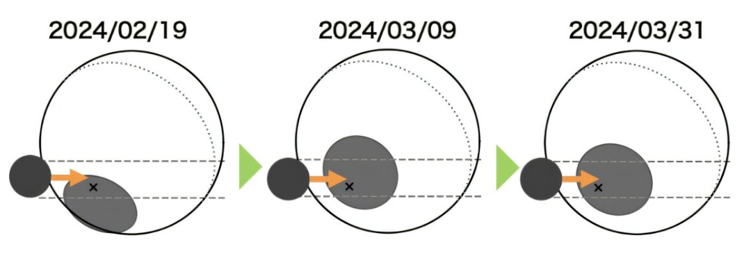
The TOI-3884 system is a unique laboratory for testing our starspot models. As seen in Figure 1, it has very convenient starspot geometry, with a large starspot located close to its pole. On top of that, we observe this star almost completely pole-on, which means that we always see this starspot, no matter how much the star rotates. To top this all off, the star hosts a close-in planet, which orbits the star from pole to pole.

Figure 1: Illustration of the TOI-3884 system. The pole (and rotation axis) of the star is indicated with a black “x,” indicating that we see the star almost pole-on. The polar starspot is indicated in grey, and the transiting planet TOI-3884b is indicated in black. Different dates are shown, illustrating how the system evolves over the span of a few weeks. [Adapted from Mori et al. 2025]

So… How Good Are Our Models?

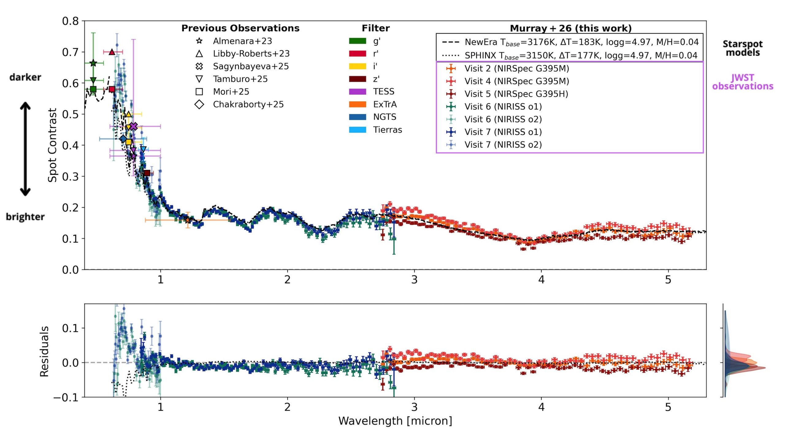
From the JWST observations, the authors extract a starspot spectrum for the first time. Figure 2 shows this as the spot contrast (how much dimmer the spot is than the surrounding stellar surface) plotted across different wavelengths. To see how well our models are doing, they compare this observed spectrum to two commonly used starspot models. The difference between the data and the models (the residual) is plotted in the lower panel.

Figure 2: The spectrum of TOI-3884’s starspot. The y-axis in the upper panel, the spot contrast, indicates how much dimmer the starspot is compared to the “normal” stellar surface. Different observations taken with JWST are indicated in different colored crosses, and other previous observations are overplotted in various other shapes. Model starspot spectra are shown in dashed or dotted black lines. The residuals between the model spectra and the JWST observations are shown in the bottom panel. [Adapted from Murray et al. 2026]

There’s still work to be done before we can confidently probe planetary atmospheres at optical wavelengths without worrying about stellar contamination, and this observed starspot spectrum provides a unique benchmark to test future starspot models. For now, the near-infrared remains a safer and more reliable window for planet atmosphere studies.

Original astrobite edited by Natalie Price.

About the author, Elise Koo:

I’m a PhD student at the University of Amsterdam, working to detect magnetic interactions between stars and their planets using radio and spectroscopic observations. Outside of research, I like to try out a variety of sports.

The post The First Starspot Spectrum Revealed by JWST appeared first on AAS Nova.

The Antennae galaxies are a nearby pair of interacting galaxies, shown in optical light from the Hubble Space Telescope (left) and in infrared light from JWST (right) in the image above. Between the two galaxies’ bright nuclei, there is a vast and dusty molecular cloud complex that harbors a large number of massive young star clusters — and in a recent article led by Rupali Chandar (University of Toledo), researchers have worked to pin down exactly how many clusters are embedded within the dusty whorls of the Antennae galaxies. The team used JWST to search for emission from star clusters too thickly blanketed with dust to be visible in previous observations by Hubble. They ultimately identified 45 sources, 40 of which were seen for the first time in this study. These star clusters mostly inhabit the overlap region between the two galaxies, are less than 2.5 million years old, and each contain roughly 10⁴–10⁶ solar masses. To learn more about how JWST’s infrared capabilities unveiled young star clusters in these interacting galaxies, be sure to check out the full article linked below.

Citation

“Nowhere Left to Hide: Uncovering All of the Massive Young Embedded Star Clusters in the Antennae with JWST,” Rupali Chandar et al 2026 ApJ 1002 64. doi:10.3847/1538-4357/ae56e8

The post Featured Image: Massive Young Star Clusters, Revealed appeared first on AAS Nova.

Discovered in December 2024, the roughly 60-meter-wide asteroid 2024 YR4 was initially thought to have a slim chance of striking Earth in 2032. Further observations ruled out an Earth impact but left open the possibility of a Moon impact. New JWST observations show that 2024 YR4 will speed past both Earth and the Moon without a collision.

Another Update on 2024 YR4

In April 2025, we featured a Research Note that described March 2025 JWST observations of 2024 YR4 and characterized the asteroid’s size and albedo. At the close of that article, the authors suggested that further JWST observations in early 2026 could help to refine our understanding of the asteroid’s trajectory and determine whether it would strike the Moon.

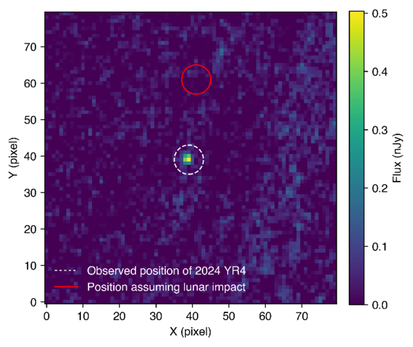
On 18 and 26 February 2026, JWST carried out those critical observations. In this dataset, the asteroid is bright enough to be detected confidently, and the background is peppered with a sufficient number of reference stars — two factors necessary to determine the precise track of the asteroid as it zipped through space.

Trajectory Refinement

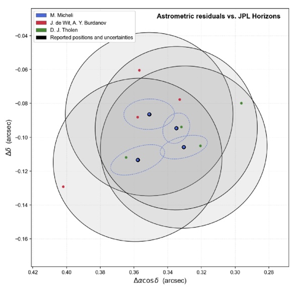
Difference between the position of 2024 YR4 determined in this work using three different reduction methods (red, blue, and green circles) and the position drawn from the existing orbit from the JPL Horizons database. The different analysis methods yielded consistent results. [Adapted from De Wit et al. 2026]

Combining the latest JWST observations with existing data stretching back to the asteroid’s discovery, de Wit and coauthors determined a new, highly precise orbit for the object — one that definitively shows that the asteroid will safely pass by the Moon at a distance of 22,900 ± 800 km in 2032. In addition to ruling out the upcoming lunar impact, the team also ruled out any collisions with Earth in the next 100 years. Phew!

Position of 2024 YR4 as seen by JWST in February 2026 (white dashed circle) compared to the asteroid’s location estimated from existing data (red circle). [De Wit et al. 2026]

High-Impact Science

This work highlights JWST’s potential as a tool for planetary defense. The February 2026 observations detailed here represent the faintest-ever detection of a near-Earth object, and JWST can detect objects far fainter than ground-based telescopes can. This ability allows JWST to observe potentially hazardous asteroids over a larger swath of their orbits, which translates to earlier trajectory estimation — JWST pinned down 2024 YR4’s orbit two years before the asteroid would have become bright enough for ground-based telescopes to do so.

JWST’s role may be even more important for smaller objects that rapidly become undetectable after discovery. De Wit’s team demonstrated this for a 10-meter-diameter 2024 YR4 clone on the same trajectory; for an object of this size, JWST would be able to rule out an Earth impact before the asteroid became undetectable, but ground-based telescopes could not. With surveys from facilities like Vera C. Rubin Observatory and Near-Earth Object Surveyor set to discover hundreds of thousands of new near-Earth objects, JWST’s role as a hazard assessor will likely be in high demand.

Citation

“JWST Observations of Asteroid 2024 YR4 Rule Out a 2032 Lunar Impact and Demonstrate a New Regime for Planetary Defense Follow-Up,” Julien de Wit et al 2026 ApJL 1003 L21. doi:10.3847/2041-8213/ae6a95

The post Asteroid 2024 YR4 Won’t Hit the Moon, New JWST Observations Show appeared first on AAS Nova.

How do massive galaxies form and evolve? A recent study traces the stellar and dust distributions across evolutionary phases of massive galaxies to better understand how massive dusty star-forming galaxies fit into the picture.

Dusty Massive Galaxies

Massive galaxies, like the Milky Way or even larger, undergo phases of active star formation and quiescent phases of inactivity, but exactly how these galaxies evolve through these stages is not yet fully understood. Dusty star-forming galaxies, which are undergoing a period of intense star formation and shrouded in dust, might be the missing evolutionary step between star-forming and quiescent phases of massive galaxy evolution. 

Currently, the leading explanation for massive galaxy formation and evolution is inside-out growth — star formation and quenching start in the inner regions of a galaxy and progress outward. However, it’s not clear whether dusty star-forming galaxies also follow the favored inside-out pathway, or if they instead proceed outside-in, first growing their disks and then assembling a central bulge.

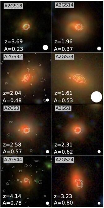
Example of JWST NIRCam images with ALMA contour lines overlaid for select dusty star-forming galaxies in the sample. [Modified from Bodansky et al 2026]

Multiwavelength Morphological Comparisons

To directly compare the star and dust morphologies across massive galaxies, Sarah Bodansky (University of Massachusetts, Amherst) and collaborators selected a sample of 33 dusty star-forming galaxies from the GOODS-ALMA 2.0 survey that searched the sky for 1.1-mm dust emission as well as star-forming and quiescent comparison samples drawn from JWST observations. Combining the ALMA survey data with JWST imaging, the authors studied the rest-frame optical (stars) and rest-frame near-infrared (dust) morphologies of dusty, star-forming, and quiescent galaxies at redshifts around cosmic noon (a few billion years after the Big Bang).

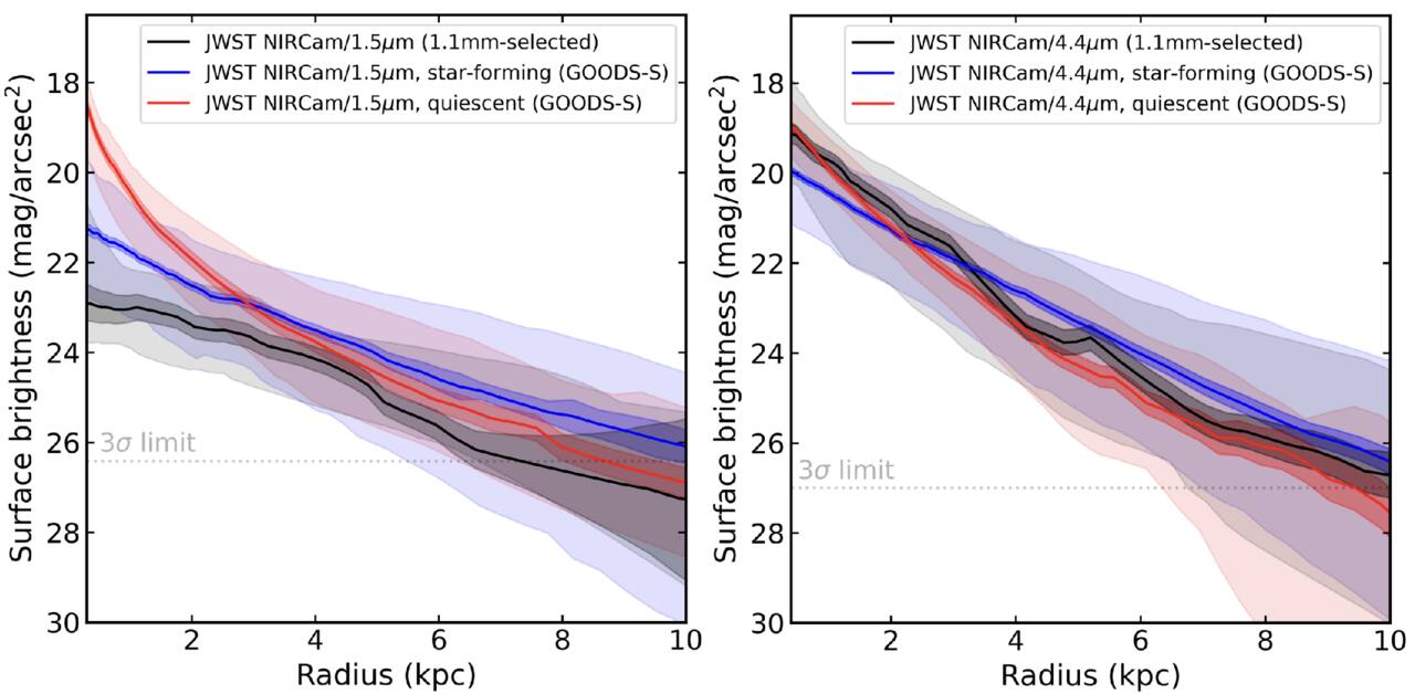
When comparing optical morphologies, the authors found that dusty star-forming galaxies and typical star-forming galaxies had similar distributions, but their near-infrared morphologies showed clear differences. Dusty galaxies tended to show more compact near-infrared emission, with dust tracing their stellar populations and more concentrated in the galaxies’ central regions. Though clearly different from star-forming galaxies, the authors noted striking similarities between the near-infrared morphologies of the dusty star-forming and quiescent galaxies, especially within their centers.

Average surface brightness profiles for the rest-optical (left) and rest-near-infrared (right) for the dusty (black), star-forming (blue), and quiescent (red) galaxies. In the near-infrared, the dusty star-forming galaxy profile appears very similar to the quiescent galaxy profile. [Bodansky et al 2026]

Citation

“JWST+ALMA Reveal the Buildup of Stellar Mass in the Cores of Dusty Star-forming Galaxies at Cosmic Noon,” Sarah Bodansky et al 2026 ApJ 1001 235. doi:10.3847/1538-4357/ae4f64

The post Hints for Massive Galaxy Evolution from Dusty Star-Forming Galaxies appeared first on AAS Nova.

Editor’s Note: Astrobites is a graduate-student-run organization that digests astrophysical literature for undergraduate students. As part of the partnership between the AAS and astrobites, we occasionally repost astrobites content here at AAS Nova. We hope you enjoy this post from astrobites; the original can be viewed at astrobites.org.

Title: Metal-Poor Star-Forming Clumps in Cosmic Noon Galaxies: Evidence for Gas Inflow and Chemical Dilution Using JWST NIRISS
Authors: Vicente Estrada-Carpenter et al.
First Author’s Institution: Arizona State University
Status: Published in ApJ

If you want to reconstruct a galaxy’s life story, one of the best “fossil records” is its metallicity. In astronomy this refers to the abundance of elements heavier than helium, which are made in stars and returned to a galaxy’s gas through winds and supernovae. Over time, more star formation usually means more metals mixed into the gas.

Now zoom to Cosmic Noon (roughly when the universe was most actively forming stars). Many galaxies in this epoch look “clumpy”; their star formation is concentrated in several bright knots scattered across the disk. The big question is where those clumps come from. Do they form from the galaxy’s own gas via internal disk instabilities, or do they light up when fresh, metal-poor gas flows in and both fuels star formation and dilutes the local metallicity?

The authors try to answer that question with JWST by measuring the metallicity of each clump relative to its immediate surroundings, rather than comparing clumps to a single galaxy-wide number (which can be misleading if the galaxy has a metallicity gradient).

They use JWST/Near Infrared Imager and Slitless Spectrograph (NIRISS) slitless grism spectroscopy from the CAnadian NIRISS Unbiased Cluster Survey (CANUCS) to study 20 lensed galaxies at redshift 0.6 < z < 1.35. (Lensing effectively acts like a zoom lens, helping to resolve smaller structures.) They focus on emission lines that trace star-forming gas, especially Hα (a star formation tracer) and sulfur lines [SII] and [SIII] (needed for their metallicity method).

Slitless spectra come with a headache: because there is no slit, different parts of a galaxy can overlap in the dispersed image. To make reliable emission-line maps from slitless data, the authors use a forward-modeling code called Sleuth, which allows the continuum to vary across the galaxy.

The authors identify clumps using the Hα map together with rest-frame ultraviolet imaging because these tracers are sensitive to star formation on different timescales: Hα highlights gas ionized by the youngest massive stars, while ultraviolet light traces young stellar light over longer periods. As a result a clump can be bright in one and not the other, especially if dust is involved.

To estimate gas-phase metallicity, they use the “strong-line” method, which infers metallicity from ratios of bright emission lines calibrated using models and empirical samples. Their main diagnostic is S23 = ([SIII] + [SII]) / Hα. Because some line ratios also depend on the ionization state (how strongly the gas is being ionized by young stars), they also use the sulfur ratio S32 = [SIII]/[SII] as a check and iterate to a self-consistent solution.

So, Are Clumps Really Chemically Different from Their Surroundings?

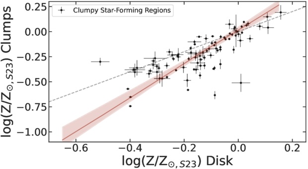
For each clump, the authors measure the metallicity inside the clump and compare it to an annulus just outside the clump (masking neighboring clumps to avoid mixing). When they plot “clump metallicity” versus “local disk metallicity,” most points fall below the 1-to-1 line, meaning the clumps are more metal poor than their surroundings (Figure 1). The mean offset is about 0.1 dex, which corresponds to roughly 20% dilution in the clump gas.

Figure 1: Each point compares a star-forming clump’s gas-phase metallicity to the metallicity of the nearby disk region immediately surrounding it. If clumps and disks had the same metallicity, they would lie on the dashed 1-to-1 line. Instead, most clumps sit below it, showing a typical ∼0.1 dex metallicity deficit, consistent with local chemical dilution. (The solid red line shows a best-fit linear trend to the clump measurement.) [Adapted from Estrada-Carpenter et al. 2025]

If inflow is really the driver, you should expect a link: the more strongly a clump is forming stars relative to its surroundings, the more diluted its metallicity should be. That is exactly what the authors find. The clumps that are most boosted in star formation are also the most metal diluted.

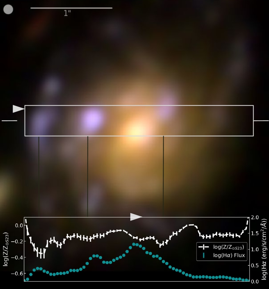
The article also emphasizes that clumps are not chemically uniform blobs. In at least one detailed example, the peaks in Hα (highest star formation) coincide with local minima in metallicity along a cut through the galaxy (Figure 2), suggesting internal star formation rate and metallicity gradients that reinforce the same story, intense star formation goes hand in hand with lower metallicity in the clump regions.

Figure 2: Example galaxy from this study illustrating the clump-scale link between star formation and metallicity. The color image shows the galaxy with a rectangular strip marking the region used for a 1D cut. In the bottom panel, the turquoise line shows the Hα flux (a tracer of recent star formation), while the white line shows the metallicity along the same cut. Peaks in Hα flux line up with local dips in metallicity, showing that the brightest star-forming clumps are also the most chemically diluted compared to nearby regions. [Adapted from Estrada-Carpenter et al. 2025]

Are These Clumps Really “In Situ,” or Could They Be Small Satellites?

A reasonable alternative is that some clumps are actually small companion galaxies projected onto the disk. These could also look metal poor, because low-mass galaxies tend to be low metallicity. The authors look for evidence using face-on systems and find that more massive clumps tend to sit closer to galaxy centers, which is consistent with in-situ clumps that form in the disk and migrate inward, though it does not rule out satellites. They argue that kinematics from JWST/NIRSpec IFU will be needed for a definitive separation.

Why This Matters

Gas inflow, star formation, and feedback, together known as the baryon cycle, are key drivers of how galaxies grow. What this article adds is a spatially resolved view that compares each clump to its local environment, showing that regions of elevated star formation also tend to be locally metal poor. That pairing is hard to explain as a simple metallicity gradient or a galaxy-wide averaging effect, and it is exactly what you would expect if at least some clumps are being fueled by relatively metal-poor inflows. In short, these clumps may be snapshots of galaxies refueling in real time.

Original astrobite edited by Ryan White.

About the author, Niloofar Sharei:

I’m an astronomy PhD candidate at UC Riverside studying how galaxies grow through star-forming clumps. I track how these clumps emerge, evolve, and sometimes survive long enough to reshape their galaxies. When I’m not thinking about cosmic blobs, I’m reading, hiking, or listening to Bach.

The post Feed the Fire, Fade the Metals appeared first on AAS Nova.

How do galaxies grow? A massive survey from JWST can help astronomers answer that fundamental question about galaxy evolution.

Time Machines

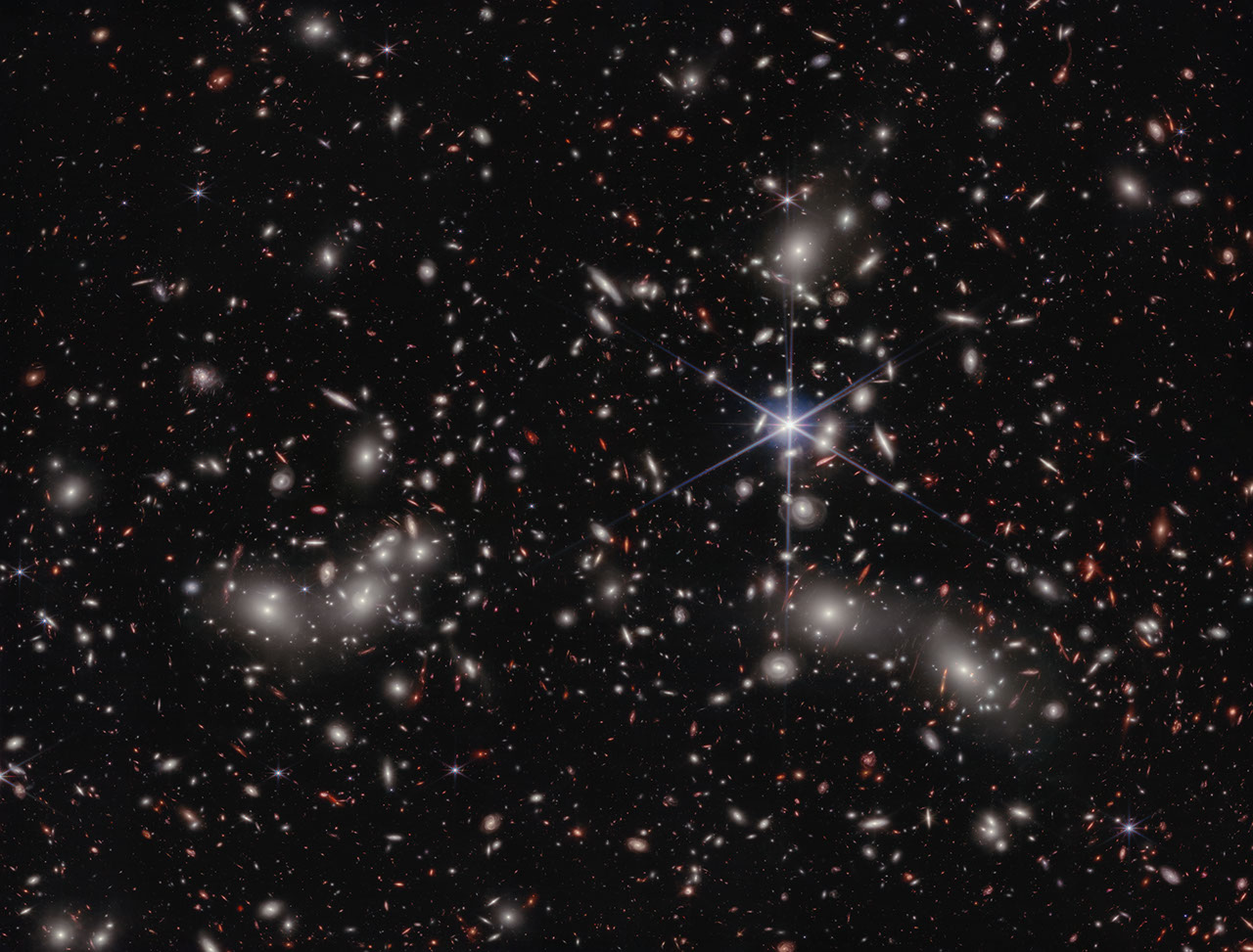
An image taken by JWST’s NIRCam instrument, the primary instrument behind the COSMOS-Web survey, of Pandora’s Cluster. Click to enlarge. [NASA, ESA, CSA, Ivo Labbe (Swinburne), Rachel Bezanson (University of Pittsburgh); Image Processing: Alyssa Pagan (STScI)]

One way astronomers could go about answering these deep, fundamental questions in galaxy evolution would be to look at many galaxies spread across different distances. Famously, since the speed of light is fairly slow (cosmically speaking), we can only see distant objects as they appeared in the past. (This is why any aliens looking toward Earth from 65 million light-years away — from within the Virgo Cluster, perhaps — would see our planet as it was when dinosaurs roamed free.) In principle, then, by looking at a progression of galaxies farther and farther away, astronomers could convert these still images into a sort of movie of how typical galaxies look moving further and further back in time.

Seeing Red

There is a complication to this strategy, however. The farther away an object is, the more the light it emits is stretched towards redder wavelengths. As a consequence, any telescope designed to detect visible light won’t see anything; to take pictures of these galaxies, we need to build detectors that are specifically sensitive to stretched-out, near-infrared light.

This is one of the primary reasons that JWST was designed, constructed, and flung into space. It was purpose-built to collect and analyze near-infrared light from distant galaxies, and now after several years of observations and data crunching, astronomers are finally getting some answers to those fundamental questions.

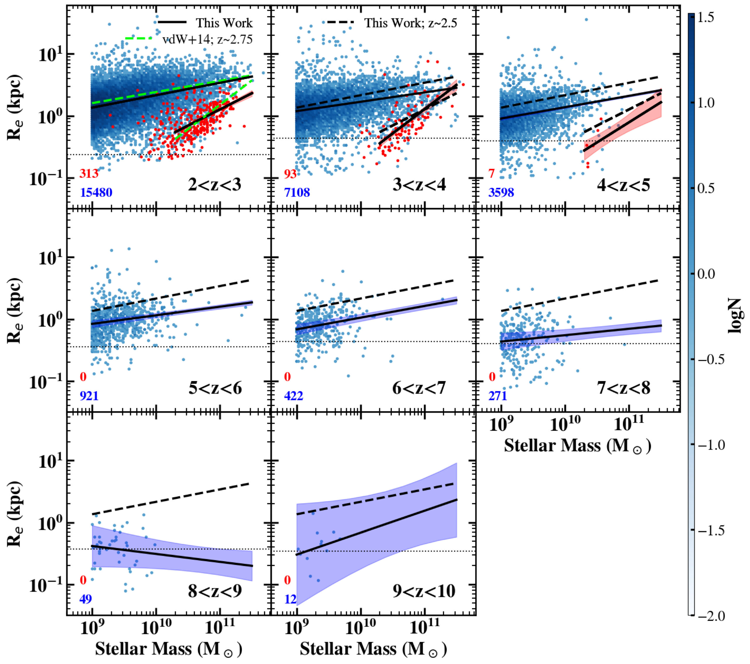
The results of how galaxies’ masses relate to their total size in different redshift bins. Click to enlarge. [Yang et al. 2025]

A Massive Survey

Recently, a team led by Lilan Yang, Rochester Institute of Technology, released their analysis of one of the earliest and largest surveys JWST has undertaken, a program called COSMOS-Web. The researchers mined a patch of sky about the size of the full Moon and extracted more than 30,000 distant galaxies, most of which had never before been seen by human eyes. They measured the brightness and size of each one and grouped them according to their redshift (a proxy for their distance) and whether they were actively forming stars or not.

The team found that, unsurprisingly, galaxies tend to grow over time. Excitingly, however, they also found that for star-forming galaxies, the relationship between a galaxy’s mass and its size is fairly constant for redshifts of z = 2–8. The scaling law between them also nicely matches up with measurements taken by the Hubble Space Telescope at smaller redshifts. Beyond that, though, for redshifts of z = 8–10, it’s possible that the scaling changes, though the authors emphasize that their sample is much smaller in these distant bins.

While more data are needed to confirm whether the youngest of these galaxies grow at a different pace than their later counterparts, we can be comforted that studies like this represent just our very first peek into a whole new era of galactic evolution, and that many more insights are sure to come as JWST keeps snapping images.

Editor’s Note: This article previously contained an error relating to the distance at which aliens would see Earth as it was when inhabited by dinosaurs. This error was corrected on 4 May 2026.

Citation

“COSMOS-Web: Unraveling the Evolution of Galaxy Size and Related Properties at 2 < z < 10,” Lilan Yang et al 2025 ApJS 281 68. doi:10.3847/1538-4365/ae0e1b

The post How Galaxies Grow Up appeared first on AAS Nova.

Editor’s Note: Astrobites is a graduate-student-run organization that digests astrophysical literature for undergraduate students. As part of the partnership between the AAS and astrobites, we occasionally repost astrobites content here at AAS Nova. We hope you enjoy this post from astrobites; the original can be viewed at astrobites.org.

Title: GLIMPSE: An Ultrafaint ≃10⁵ M_⊙ Pop III Galaxy Candidate and First Constraints on the Pop III UV Luminosity Function at z ≃ 6–7
Authors: Seiji Fujimoto et al.
First Author’s Institution: University of Toronto; The University of Texas at Austin
Status: Published in ApJ

You, me, your laptop, my $8 matcha, and just about everything else on Earth was forged in the fiery bellies of dying stars. Generations of stars had to live and die before the universe became enriched with any elements heavier than helium (what astronomers call “metals”). The first stars to undergo this cosmic cycle are known as Population III (Pop III) stars. Though their existence has been hypothesized since the 1960s, astronomers have failed to observe these distant metal-free stars or the faint, low-mass galaxies that host them.

The first Pop III stars likely formed around 100 million years after the Big Bang in pristine pockets of hydrogen gas. Although these are too distant for us to observe, we expect that as the universe started to become metal enriched, there were still existing pockets of gas introverted enough to survive unpolluted and form metal-free Pop III stars up to a redshift of z ~ 6–7 (when the universe was around 900 million years old)!

JWST is the perfect instrument to search for these systems. You can read other astrobites on the search for possible Pop III systems with JWST here and here. The authors of today’s article seek to develop the most efficient way of using JWST’s Near-Infrared Camera (NIRCam) to find the galaxies hosting Pop III stars. Using their selection method on existing NIRCam data, the authors identified one promising Pop III galaxy candidate.

I’m Not Like Other Galaxies

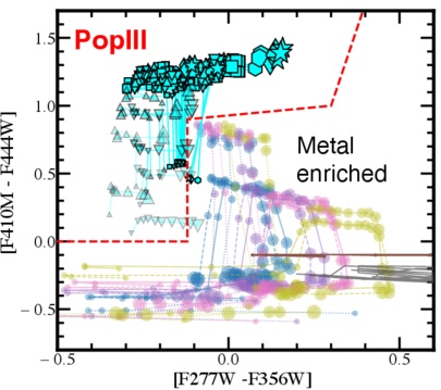
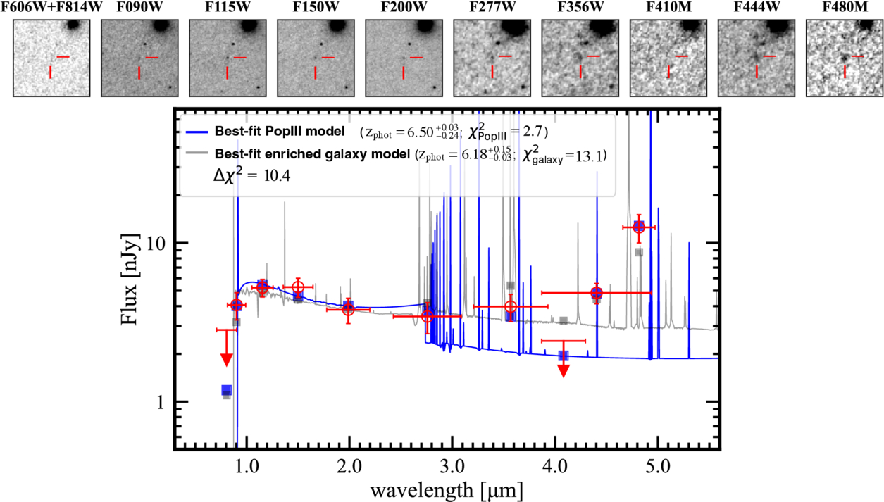
In order to find a Pop III galaxy, we need to take a look at galaxies’ spectral energy distributions (SEDs). These are graphs that show the energy emitted by a galaxy at different wavelengths of light. Pop III galaxies are expected to have SEDs that differ from your everyday, metal-enriched galaxy. NIRCam will be especially sensitive to three key spectral features that show up in the SEDs of Pop III galaxies: an absent [O III] line (light emitted by doubly ionized oxygen atoms), a strong H-alpha line (light emitted when a hydrogen atom transitions from its third to its second energy level), and a significant Balmer jump (light absorbed to ionize electrons in the second energy level of a hydrogen atom). To identify these key SED characteristics, the authors use SED fitting and color–color diagrams to execute an efficient Pop III search with NIRCam.

The first selection method involves SED fitting. Astronomers create template SEDs that represent different types of galaxies and then compare these templates to the observed SEDs to see which one matches best. In this work, the authors use metal-rich galaxy templates and Pop III templates to fit the galaxies observed with NIRCam. They then calculate the chi-squared χ² (a statistical measure of best fit) between the data and all the SED templates. A galaxy is selected as a Pop III candidate if the Pop III model provides a good fit (χ² < 10) to the photometry and is significantly better than any metal-rich model. It’s kind of like looking for Cinderella by making every woman in the kingdom try on the glass slipper.

Figure 1: Color–color diagram for selecting Pop III galaxies where the x and y-axes show the different NIRCam filters being subtracted. The cyan symbols are different Pop III models while the other colored dots are different metal-rich galaxy models. [Adapted from Fujimoto et al. 2025]

O Pop III, Pop III, Wherefore Art Thou?

The authors apply their fresh new selection criteria to publicly available NIRCam data from large surveys. And (drum roll please) the slipper fits! The Pop III galaxy candidate GLIMPSE-16043 is an ultra-faint galaxy at z = 6.5. It was imaged in the GLIMPSE survey, which uses the technique of gravitational lensing to observe faint and distant galaxies.

The GLIMPSE survey targeted a massive galaxy cluster, Abell S1063. The cluster bends the light from distant galaxies and, like a giant lens, magnifies faraway objects, providing some of the deepest JWST imaging to date. The Pop III candidate passes both tests: it resides in the Pop III region of the color–color diagram, and its SED is best fit by a Pop III model, not a metal-rich galaxy model (see Figure 2). Next, spectroscopic follow-up is needed to ensure that this galaxy is truly metal free and not just extremely metal poor.

Figure 2: SED of GLIMPSE-16043 with the best-fit Pop III template (blue) and best-fit metal-enriched template (gray). The top panel is the galaxy imaged in different filters from NIRCam and the Hubble Space Telescope. [Fujimoto et al. 2025]

Original astrobite edited by Chris Layden and Margaret Verrico.

About the author, Madison VanWyngarden:

I am a first-year PhD student in astronomy and NSF Graduate Research Fellow at the University of Arizona. I study galaxy formation and evolution in the distant universe and am particularly interested in dusty star-forming galaxies. In my free time, I love reading, hiking, and baking bread!

The post A Possible GLIMPSE of the Universe’s First Stars appeared first on AAS Nova.