
❌

Reading view

The search for habitable worlds

The NASA Exoplanet Exploration Program (ExEP) has a curated list of 164 nearest Sun-like stars that are easily visible from Earth. This list represents the first targets for a proposed large space telescope specially designed to find life in the universe, currently known as the Habitable Worlds Observatory (HWO). 

After the HWO is completed, likely sometime in the 2040s, scientists will use the specialized telescope to directly image planets in those star systems. The telescope will search around Sun-like stars for planets in a region known as the habitable zone, where temperatures allow liquid water to exist. Scientists hope to find Earth-like planets with liquid water in the habitable zones of other stars.

While the 164 stars on ExEP’s list have qualities that make them good candidates for study, it remains unknown how many actually have terrestrial planets within their habitable zones. A team of scientists at Arizona State University used simulated data for ExEP’s 164 stars and their hypothetical planetary systems to assess which are most likely to have habitable worlds. Their results would help the HWO prioritize which star systems to observe.

The team started with a subset of 134 stars on ExEP’s list with no known exoplanets, giving researchers the freedom to simulate potential worlds around them. They used a software model called the DYNAmical Multi-planet Injection TEster (DYNAMITE) to predict the possibility that an unseen planet exists around each star by generating 100,000 simulated planetary systems around it. The simulations use mathematical formulas based on observations of real exoplanets to determine the sizes and orbital characteristics of hypothetical gas giants and rocky exoplanets. DYNAMITE then determines whether these planetary systems would be stable and include a terrestrial exoplanet in the star’s habitable zone.

The other 30 stars in the ExEP’s list have known exoplanets, but none of them are rocky planets in habitable zones. To predict whether these stars have unseen terrestrial planets in their habitable zones, the team used the same DYNAMITE process as before with the additional requirement that each star must have an exoplanet matching the one already found.
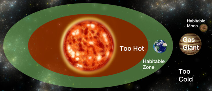
The space around a Sun-like star can be divided into three regions. The region closest to the star is too hot for liquid water to persist on an exoplanet’s surface, while the region farthest from the star is so cold that any water on an exoplanet would be frozen solid. Between these lies the habitable zone, where temperatures would allow liquid water to exist. However, it’s also possible that a combination of light and gravity could create habitable temperatures on large enough moons orbiting gas giants even beyond a star’s main habitable zone. Illustration by <a href="https://www.linkedin.com/in/andrew-bizal-ab14401ab/">Andrew Bizal</a>.

The space around a Sun-like star can be divided into three regions. The region closest to the star is too hot for liquid water to persist on an exoplanet’s surface, while the region farthest from the star is so cold that any water on an exoplanet would be frozen solid. Between these lies the habitable zone, where temperatures would allow liquid water to exist. However, it’s also possible that a combination of light and gravity could create habitable temperatures on large enough moons orbiting gas giants even beyond a star’s main habitable zone. Illustration by Andrew Bizal.

To increase the chances of finding a terrestrial planet in a habitable zone, the team also investigated potentially habitable moons orbiting gas giants in these systems. For each simulation that included a gas giant, the team inserted between 2 and 23 moons, with masses between 10% of Earth’s Moon and 50% of Earth. Then they simulated the surface temperatures of these moons based on how much starlight they receive and how strongly their host planet pulls on them. They deemed the moons potentially habitable if they were large enough to retain an atmosphere and had a temperature ideal for liquid water, even if they were not technically in their stars’ habitable zones.

For each star, the team calculated a metric based on the probabilities that the star had a terrestrial planet in its habitable zone, that the planet would remain in a stable habitable zone for at least 2 billion years, and that the star had a potentially habitable moon. They called this probability statistic a ranking metric and used it to compare star systems. 

Based on the ranking metric, the team found that the dimmer and cooler stars on their list generally had better chances of hosting a habitable-zone terrestrial planet than the brighter, hotter stars. They also found that stars without known exoplanets ranked more favorably. Around 70% of the stars with known exoplanets had less than a 1% probability of hosting a terrestrial planet in their respective habitable zones. Additionally, fewer than 0.1% of their simulated moons were habitable.

Overall, the researchers concluded that the HWO should prioritize observing cooler, Sun-like stars with no known exoplanets. They claimed that the exoplanets with known characteristics in their sample set were of sizes and in positions that made it unlikely for other exoplanets to be in their systems’ habitable zones. Even with expanded habitability criteria for moons, it would be very unlikely for HWO to find another Earth orbiting a gas-giant exoplanet. They ranked 47 stars in the highest-priority category (A Tier), 51 stars in the middle category (B Tier), and 66 stars in the lowest category (C Tier) to observe with HWO. 

At the end of their study, the team remarked that the proposed HWO represents a potential next step in the search for other Earths, but scientists still need to identify the best targets for this future telescope. The HWO telescope should be able to image rocky exoplanets directly, so thorough research to prepare a list of high-priority targets will help avoid overlooking other Earths.

The post The search for habitable worlds appeared first on Sciworthy.

  •  

Where did the galaxy get its carbon?

Carbon is the 4th most abundant element in the universe. It’s everywhere, from the air you breathe to the carbohydrates in your food to the petroleum in the Earth’s crust. Like most elements, carbon was not created by the Big Bang, but came from 2 different types of stars that fuse lighter elements together. 

Massive stars at least 8 times the Sun’s mass fuse 3 helium atoms into a carbon atom in their cores, through a mechanism called the triple-alpha process. They eventually expel this carbon into space, either through a stream of material called a stellar wind or at the end of their lives during a core-collapse supernova. 

Meanwhile, low-to-intermediate-sized stars between ½ and 8 times the Sun’s mass also induce the triple-alpha process. But unlike massive stars, they produce carbon not in their cores, but in a dense shell of helium that surrounds them during an advanced stage known as the asymptotic giant branch or AGB. AGB stars undergo cycles of swelling and contraction, during which they shed some of their material into space.

While scientists understand these processes, the contribution of each star type to the carbon supply in the universe remains uncertain. To address this, a team of scientists modeled how the chemical elements in the Milky Way Galaxy change over time with different contributions from the 2 carbon-creating processes. They then verified their findings by comparing them with the actual carbon concentration in the Milky Way.

To obtain the benchmark for the Milky Way Galaxy’s carbon content, the team turned to the catalog of stars observed by the Apache Point Observatory Galactic Evolution Experiment (APOGEE) survey. They selected 14,066 stars that were large and bright enough to yield reliable data but, unlike AGB and massive stars, were still at a stage of life when their newly produced carbon was still confined to their cores. The researchers used the carbon in the outer layers of these stars, known as subgiants, as a compositional record of the gas from which they formed, thereby estimating the Galaxy’s carbon content during their formation. 

The scientists started with a computer program developed by another team that models how the Milky Way’s chemistry changes over time. First, the team calculated the potential amount of carbon produced by different types of stars using estimates from earlier studies. Then, they incorporated these results into a model that accounts for how stars form, fuse elements, and release carbon into the Galaxy, using a simulation program called the Versatile Integrator for Chemical Evolution, or VICE. The researchers ran 14 versions of this model, each assuming a different contribution of carbon from AGB stars relative to massive stars.

In their computer model, the Milky Way Galaxy began as a set of 200 concentric rings, each containing its own population of stars, different speeds at which stars form, and varying amounts of gas available to form new stars. The team then stitched these rings together by having stars migrate between them. They allowed these model Galaxies to settle over 10 billion years, then picked a random sample of 14,066 simulated stars to compare their carbon content with carbon in the same number of observed subgiants from APOGEE.

The team’s model most closely reproduced the actual carbon content of the Milky Way’s subgiant stars when AGB stars contribute between 10% and 40% of the Galaxy’s carbon, with the strongest agreement occurring at 15% to 30%. Even though they found that massive stars are the dominant source of carbon, they also found that smaller AGB stars could produce carbon more efficiently than previously thought, though they take longer to become carbon sources than their larger counterparts.

The team concluded that their estimates of how much carbon comes from AGB and massive stars provide a benchmark for future studies, as the connection between the production of elements inside stars and the processes by which those same stars lose mass remains poorly understood. They suggested that future researchers analyze larger sample sizes, examine other galaxies, and use data from future surveys to better understand the chemical history of the universe.

The post Where did the galaxy get its carbon? appeared first on Sciworthy.

  •  

NASA’s Roman Space Telescope Now Has Fuel for at Least 22 Years

Roman Telescope’s 22-Year Fuel Supply NASA fitted the Nancy Grace Roman Space Telescope with a grapple fixture and

💾

Auf YouTube findest du die angesagtesten Videos und Tracks. Außerdem kannst du eigene Inhalte hochladen und mit Freunden oder gleich der ganzen Welt teilen.
  •  

Objects at the border between planets and stars

Beyond the solar system, the line between planet and star can get blurry. Astronomers call objects that fall between the size ranges of planets and stars substellar objects. One type of substellar object, called a brown dwarf, forms from collapsing gas clouds like a star, but is not quite massive enough to fuse hydrogen in its core. Some can briefly fuse a heavier form of hydrogen, known as deuterium, in their cores, though never enough to produce starlight. Others are small and cold enough to develop complex atmospheres.

Recently, astronomers discovered a new type of substellar object in a star-forming region of the Milky Way Galaxy called IC 348. Using observational data from the JWST’s Near InfraRed Spectrograph (JWST NIRSpec), they found objects 0.2% to 1.2% the mass of the Sun that float freely like stars but have carbon-containing molecules called hydrocarbons in their atmospheres. Because these objects are smaller than known brown dwarfs and have evidence of hydrocarbons, scientists refer to them as H-type objects.

To investigate what H-type objects are and where they fit within the spectrum of substellar objects, researchers Richard J. Parker and Catarina Alves de Oliveira analyzed survey data on stars and substellar objects in IC 348, then conducted follow-up simulations to uncover how H-type objects formed. The main question they asked was whether H-type objects form from collapsing gas clouds, like brown dwarfs and stars, or develop around host stars before being ejected and drifting freely through space, like planets.

First, they reviewed the observational records of IC 348 obtained with the JWST NIRSpec and the near-IR spectrograph SpeX at the NASA Infrared Telescope Facility. IC 348 has 495 stars and brown dwarfs combined, as well as 9 H-type objects. Estimates for the age of this star-forming region range from either 1 to 3 million years or 5 to 6 million years, depending on how different teams calculated it. From there, Parker and Alves de Oliveira compared where the stars, brown dwarfs, and H-type objects were located within the cluster. They found no unique spatial distribution among the 3 types of objects.

Then, the team simulated the evolution of IC 348 over 10 million years to determine which initial conditions would result in a spatial distribution closest to the survey data. They simulated an initial giant gas cloud and used a mathematical function to distribute its mass among the 495 constituent objects. The researchers then placed a Jupiter-sized planet around each simulated star that was approximately the Sun’s mass to determine whether they could grow and escape their home star and become H-type objects. They also repeated the simulations by placing the Jupiter-sized planets at distances from the Sun similar to those of Earth, Jupiter, and Neptune, and varied the sizes and star densities of the simulated IC 348 regions.

They found that if Jupiter-sized planets orbited their stars at roughly Jupiter’s distance from the Sun, then 5 to 15 of them could escape their stars in a region like IC 348, which would roughly match the number of known H-type objects. However, the escaped planets were distinctly more spread-out than the observed H-type objects, which share a similar spatial distribution with the cluster’s stars and brown dwarfs. Since the simulations did not match the observed distribution, the researchers suggested that these H-type objects are likely a new sub-category of very small brown dwarfs rather than escaped planets.

Although this study favors a brown dwarf origin for H-type objects, the exact details of how they formed remain up for debate. Astronomers still have multiple competing theories about how ordinary brown dwarfs form. Perhaps they are ejected from their gas cloud before fully forming, have their outer layers stripped by radiation from a nearby massive star, or simply form like stars on a slightly smaller scale. Regardless, future researchers will continue to explore this murky area of substellar astronomy.

The post Objects at the border between planets and stars appeared first on Sciworthy.

  •  

Characterizing galaxies at “cosmic noon”

The universe is around 14 billion years old, but scientists theorize that no stars formed for the first several hundred million years, during an era known as the cosmic dark ages. They refer to the first billion years or so after this, when stars formed, as the cosmic dawn. At that time, the very oldest galaxies first assembled from collections of gas and plasma. 

As these galaxies assembled and more material became available, the number of stars formed each year increased. Around 2 to 3 billion years after the Big Bang, galaxies grew faster than they ever would, producing stars at the highest rate in the universe’s history. This era is called cosmic noon.

Researchers from the Netherlands recently investigated 3 distant galaxies whose light began its journey to Earth during cosmic noon. They selected targets from a set of ancient star-forming galaxies identified in the ALMA – Archival Large Program to Advance Kinematic Analysis or ALMA-ALPAKA project. Of these, they chose to study 3 galaxies labeled ID1, ID3, and ID13.

They combined 2 different types of data to produce a detailed description of these galaxies. First, they collected data from an enormous telescope comprising 66 antennas in Chile, known as the Atacama Large Millimeter/submillimeter Array or ALMA. They used ALMA to detect radio-wave emissions from carbon monoxide and elemental carbon in these galaxies. The researchers stated that studying these chemicals in distant galaxies could reveal how their free-floating gas clouds move. They also used publicly available data from JWST’s Near Infrared Camera, or NIRCam, to determine how much light the galaxies’ stars emitted. By analyzing cosmic noon galaxies in multiple different ways, the team aimed to measure their masses and the relative contributions of regular matter and dark matter.

They used a computer program developed by other astronomers to interpret the JWST data as a series of maps showing the distribution of stars across each galaxy. They used this light-emission data to estimate the total mass of all the stars in these galaxies. Then they developed an original computer program to map the distribution of gas through each galaxy using the ALMA data. The team used these maps to create plots, known as rotation curves, which show how fast particles orbit each galaxy’s center as a function of their distance from it. 

The astronomers used these rotation curves to estimate the amount of dark matter in each galaxy. They explained that this method works because dark matter is totally invisible, but it still exerts a gravitational pull. Its gravitational pull causes visible material like stars and gas closer to the edges of these galaxies to move faster than they would in galaxies without dark matter. 

The team found that these galaxies had between 39 and 80 billion times the mass of our sun, or solar masses, in stars. They had between 4 billion and nearly 16 billion solar masses worth of free-floating gas. And they had from 1 trillion to 31 trillion solar masses of dark matter.

However, when the team compared the light-emission data with the rotation curves, they found a discrepancy. Typically, dark matter resides in a shell or halo surrounding a galaxy, meaning it should mostly affect material near the galaxy’s outer edge. Since astronomers don’t usually have to account for dark matter near a galaxy’s center, they can calculate the total mass of center material based on the amount of gas and stars they see there. But near the centers of these galaxies, the team found that the masses they derived from the light emissions were less than what they calculated from the rotation curves. 

They proposed multiple potential explanations for this discrepancy. First, they suggested that the halo shape might not be a good model for the dark matter distribution in all galaxies, meaning that cosmic noon galaxies could contain dark matter near their centers. Second, they suggested that stars could be packed tightly in the center of these galaxies, blocking each other’s light emissions. Third, they suggested that galaxy ID1 could have a supermassive black hole as big as 1.5% its total stellar mass at its center.

The team concluded that they now have a detailed picture of the mass distribution in these cosmic noon galaxies, but the reason for their center mass discrepancies remains elusive. They suggested that a complex relationship exists between the dark matter halos and the rest of the material within these galaxies. They indicated that future astronomers could adapt their methods to study the distribution of material in other distant galaxies studied by ALMA-ALPAKA and forthcoming galactic surveys.

The post Characterizing galaxies at “cosmic noon” appeared first on Sciworthy.

  •  
❌