❌

Reading view

Between 1989 and 1997 the United States shipped more than 50 million pet turtles abroad, and enough of the red-eared sliders were later dumped in ponds and rivers when they grew too big that the species now outcompetes native turtles on every continent but Antarctica, listed among the 100 worst invaders on Earth.

The story begins with a cartoon. In late 1987 a low-budget animated series called Teenage Mutant Ninja Turtles began airing on American children’s television, and within eighteen months it had become the most successful children’s franchise of its decade. Sales of turtle-themed toys, lunchboxes, video games, and Halloween costumes went through the roof. And so did sales of actual pet turtles. American reptile farms, most of them clustered along the Mississippi River basin where the red-eared slider is native, ramped up production to meet the demand. Hatchlings the size of a fifty-cent piece were shipped by the tens of millions to pet stores across the United States and around the world.

What almost nobody selling the turtles bothered to mention was that a hatchling red-eared slider grows into an adult red-eared slider weighing up to three kilograms, requiring a hundred-gallon tank with filtration, and living for forty years or longer. Within a few years, unwanted adult sliders started turning up in ponds, rivers, and public parks in countries where the species had never existed before.

How 52 million turtles left the country

According to the International Union for Conservation of Nature’s Global Invasive Species Database entry on Trachemys scripta elegans, compiled by the IUCN Species Survival Commission’s Invasive Species Specialist Group and citing the original Telecky 2001 tally of the United States pet turtle export trade, more than 52 million red-eared sliders were exported from American turtle farms to overseas pet markets between 1989 and 1997. The primary destination was China, though large numbers also went to Japan, Taiwan, Thailand, South Korea, and Singapore, along with substantial shipments to France, Spain, Italy, Germany, the United Kingdom, Australia, South Africa, and Brazil. The reason American farms could produce sliders at that scale was that the species is remarkably easy to breed in captivity. The reason they were so easy to ship was that a hatchling turtle weighs almost nothing and can be packed into ventilated boxes by the hundreds.

The European Union, watching this happen in real time, banned the import of Trachemys scripta elegans on 22 December 1997. That single regulatory decision effectively ended the American export trade to Europe overnight. By the time it came into effect, however, the damage across the European continent was already done. Feral populations had established themselves in France, Spain, Italy, Portugal, Slovenia, Greece, Germany, Austria, Switzerland, the Netherlands, Belgium, Poland, Latvia, and the United Kingdom. Similar populations were showing up in the wetlands of every country the trade had reached. The turtles that had already been sold were still alive. Their owners were still tiring of them. The ponds behind their houses were still available.

If our animal kingdom fascinates you, you’ll enjoy this video we made on the recorded adventure of a young elephant bull, and what his route revealed: 

What happens when a tank turtle meets a lake

The red-eared slider turns out to be an unusually well-equipped invader. It reaches sexual maturity in three to four years, which is faster than most native freshwater turtles it competes with. Females can lay up to six clutches per year of up to thirty eggs each, giving the species a reproductive rate roughly two or three times higher than the European pond turtle it is now displacing across much of the continent. Adults tolerate a wide range of water conditions, from clean rural rivers to heavily polluted urban canals. They are omnivorous and will eat almost anything a freshwater environment can offer. They are aggressive at basking sites and will physically displace smaller native turtles from the sunning logs they need for thermoregulation.

The competitive dynamic has been most extensively studied in France, where researchers from the University of Paris-Sud have been documenting the interaction between introduced sliders and the native European pond turtle (Emys orbicularis) for the past two decades. What they have found is that in ponds where sliders are present, the native pond turtles are pushed to lower-quality basking sites, tend to survive at lower rates, and produce fewer offspring per breeding season. The European pond turtle is classified as Near Threatened on the IUCN Red List. Every additional slider in a European wetland adds to the pressure. Similar competitive displacement has been documented in Washington State against the Pacific pond turtle, in Australia against native short-necked turtles, and across Asia against a dozen freshwater species that had evolved in the absence of anything resembling a Mississippi-basin generalist.

According to The Nature Conservancy’s 2019 Cool Green Science article on American species invading other countries, written by staff science journalist Justine E. Hausheer, the geographic reach of the red-eared slider now covers essentially every continent where freshwater habitat and moderate temperatures exist. Established feral populations have been confirmed in the western United States, Australia, New Zealand, Europe, Great Britain, South Africa, the Caribbean, the Middle East, Southeast Asia, and several Pacific island groups. Only Antarctica remains slider-free, and even that exemption is only because Antarctica has no freshwater ponds and does not get above freezing for most of the year. If it did, and it had ponds, the sliders would probably be there too.

The IUCN Species Survival Commission’s Invasive Species Specialist Group formally listed the red-eared slider on the Global Invasive Species Database’s roster of the hundred worst invasive species anywhere in the world. The species now ranks number 93 on that list. It sits alongside brown rats, feral cats, cane toads, and the emerald ash borer as a species whose global spread has caused measurable and lasting ecological harm. Australia’s Vertebrate Pests Committee has assigned it a threat category of EXTREME. Multiple European countries have banned its sale, its keeping as a pet, or both. Illegal shipments continue anyway. Buddhist mercy ceremonies in parts of East Asia continue to release captive-bred sliders into rivers as an act of religious devotion, unaware or unbothered that the specific animal being released is an invasive species that will outcompete the native turtles the ceremony was originally designed to protect.

What the whole episode represents is one of the more improbable ecological consequences of a late-1980s children’s television programme. The Ninja Turtles cartoon ran for ten years. American reptile farms produced tens of millions of live turtles to meet the resulting demand. The turtles grew larger than their owners expected. The owners released them into the nearest available water. And forty years later, a native North American reptile that once occupied the freshwater ponds of a few states along the Gulf Coast now occupies almost every freshwater pond on the planet warm enough to support it. The turtles never asked to be there. They just weren’t given much choice. And once they arrived, they turned out to be remarkably well-suited to staying.

The post Between 1989 and 1997 the United States shipped more than 50 million pet turtles abroad, and enough of the red-eared sliders were later dumped in ponds and rivers when they grew too big that the species now outcompetes native turtles on every continent but Antarctica, listed among the 100 worst invaders on Earth. appeared first on Space Daily.
  •  

Astronauts on the space station have no washing machine, because water is far too precious to waste on laundry, so they wear the same clothes for days and then pack the dirty ones into a cargo capsule that burns up on reentry, which means a fireball crossing the sky could, in theory, be a bundle of an astronaut’s old underwear.

The International Space Station has been in continuous crewed operation since November 2000, which means somebody has been living roughly four hundred kilometres above the surface of the Earth every single day for the past twenty-five years without a break. During that time the station has been visited by more than two hundred and eighty astronauts and cosmonauts from more than twenty countries, and each of them has faced the same practical problem that any long-term resident of anywhere eventually has to solve.

Their clothes get dirty. And the space station, for reasons that come down to the physics of orbital resupply, does not have and has never had a washing machine on board. What NASA and the Russian space agency have therefore developed over the intervening decades is one of the more counterintuitive laundry solutions in any modern human institution. There is no laundry. The clothes go into a cargo capsule when the astronauts are done with them. The cargo capsule burns up on the way home.

Why nobody bothered to send a washing machine up

The reason is water. Aboard the space station every drop of water is a precious resource that either has to be lifted up from Earth at roughly $10,000 per kilogram in launch costs, or has to be extracted and recycled from the crew’s own urine, sweat and exhaled breath through a purification system that operates continuously in the background of station life. The station recycles roughly 90 per cent of the water it produces internally, which is considerably better than any comparable industrial recycling system on Earth. But even at that recycling rate, adding a washing machine to the water demand of the station would consume enough additional water per cycle to fundamentally change the economics of resupply. According to a 2017 VICE interview with Robert Trevino, a senior engineer with NASA’s Crew and Thermal Systems Division who is responsible for astronaut clothing on the station, the engineering team has been examining this question for years. NASA’s own internal trade studies compared the water and power requirements of a hypothetical station laundry system against the cost of simply replacing dirty clothes with fresh ones sent up on cargo runs. Replacing the clothes turned out to be cheaper. So that is what NASA does.

If space exploration fascinates you, you’ll enjoy this video we made on why astronauts come home feeling like they’re being watched…

What this means in practical terms is that astronauts on the station wear each piece of clothing for as long as it can reasonably be worn before it becomes unusable. Exercise clothes get roughly two weeks of use because the mandatory hour of daily exercise required to prevent bone and muscle loss in microgravity produces enough sweat to defeat the antibacterial coating on the fabric within a fortnight. Regular daily-wear clothes, meaning the cotton polos and cargo shorts that most station astronauts prefer, get anywhere between one and three months of wear per garment. Underwear rotation is up to the individual crew member. Trevino told VICE that former astronaut Don Pettit was known to have worn the same pair of shorts for months at a stretch, which was apparently a source of considerable amusement among his crewmates. The clothing is sourced by NASA’s contractor Lockheed Martin from ordinary commercial suppliers, including Lands’ End, Cabela’s, and Blackhawk. There is nothing technologically special about the fabric.

Where the clothes actually end up

Once a garment has reached the end of its useful wearing life, it goes into the station’s waste system alongside the packaging, food waste, expired equipment, and general trash that the crew generates every day. The waste is bagged, taped, and stored in whichever visiting cargo vehicle happens to be docked at the time. There are currently three different cargo vehicles that regularly deliver supplies to the station. Russia’s Progress capsule and Northrop Grumman’s Cygnus vehicle are both single-use, meaning they are launched from Earth full of supplies, unloaded at the station, refilled with trash, undocked, and then deliberately deorbited over the Pacific Ocean where they burn up in the upper atmosphere on the way down. SpaceX’s Dragon capsule is the exception. It is reusable, and it returns to Earth intact via parachute for a splashdown in the Pacific and eventual reuse on a subsequent mission. So while Dragon comes home in one piece, the trash from every Progress and Cygnus run ends up as a spectacular fireball crossing the sky somewhere in the upper atmosphere above the South Pacific.

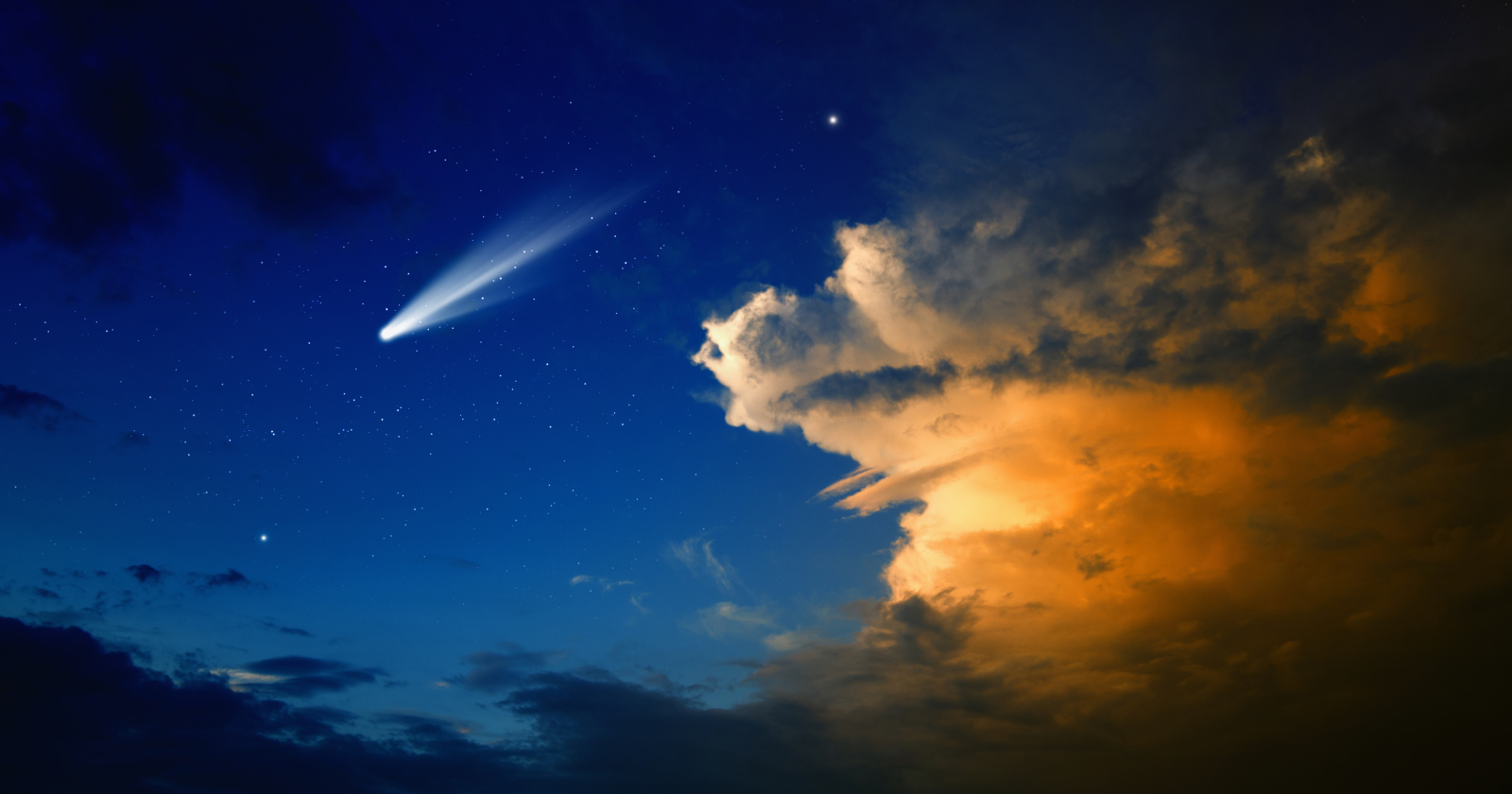
According to Space.com’s November 2023 reporting by managing editor Brett Tingley on the reentry of the Russian Progress MS-23 cargo spacecraft, the reentry of a fully loaded trash-carrying capsule is a visually striking event. The Progress MS-23 undocked from the station on 29 November 2023 carrying, in the words of the Roscosmos cosmonaut Oleg Kononenko who saw it off, “old equipment and household waste, or everything the experts have decided to toss from the station.” Four hours later NASA astronaut Jasmin Moghbeli, who had been alerted by mission control to look out of a specific window at a specific time, was able to photograph the reentry from the ISS itself. Her photographs show what looks like a spectacular meteor. Bright trails of fire streak across the darkness of the upper atmosphere. The main capsule breaks apart into several distinct fragments as the atmospheric heating destroys its structural integrity. Then everything disperses into smaller and smaller sparks until nothing recognisable is left. Moghbeli wrote on X afterwards that the whole event lasted only two or three minutes and reminded her of fireworks.

What was inside the capsule during those two or three minutes was, among many other things, the accumulated clothing that seven astronauts and cosmonauts on the station had been wearing over the preceding several months. Somewhere in the fireball was Kononenko’s old exercise gear, along with the daily-wear cotton polos of the American, Japanese, and Danish crew members who had been aboard during the same period. Whether any of the specific garments in question had been observed by anyone on the ground as bright flashes in the night sky is impossible to say with certainty. But the fireball that briefly crossed the upper atmosphere above the South Pacific on the evening of 29 November 2023 did in fact contain, among its many other contents, the discarded underwear of at least seven people who had been living in low Earth orbit at the time.

Which is to say that the surprising claim in the title turns out to be more or less exactly what actually happens. The station has no washing machine. The clothes get worn until they can’t be worn any longer. They get packed into whichever cargo vehicle is next scheduled to depart. And the cargo vehicle, on its final trajectory back through the upper atmosphere, becomes a briefly visible streak of light in the night sky before the whole thing burns away to nothing over the Pacific Ocean. If you happen to be looking up at the right moment from the right latitude, and if you know the timing of the current Progress or Cygnus deorbit schedule, you might catch one. And what you would be watching, in the strict literal sense, is somebody’s old socks and shirts on their final journey home.

The post Astronauts on the space station have no washing machine, because water is far too precious to waste on laundry, so they wear the same clothes for days and then pack the dirty ones into a cargo capsule that burns up on reentry, which means a fireball crossing the sky could, in theory, be a bundle of an astronaut’s old underwear. appeared first on Space Daily.
  •  

In 1984, NASA left a satellite carrying 57 experiments in orbit for a planned 10 months — repeated delays stretched the trip to 69 months before Columbia brought the entire laboratory home inside its cargo bay, its exposed surfaces weathered by years in space.

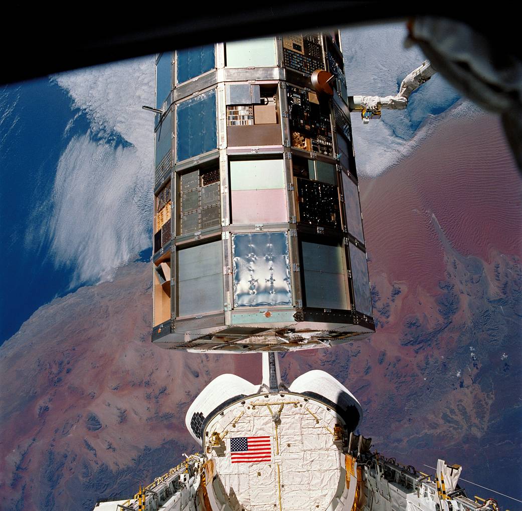
The experiment-covered Long Duration Exposure Facility held by the shuttle robotic arm above Columbia’s payload bay

When NASA deployed the Long Duration Exposure Facility in April 1984, its experiments were supposed to spend about ten months in orbit before returning to Earth. Instead, scheduling changes and the aftermath of the Challenger accident extended the flight to 69 months. Columbia finally collected the facility in January 1990 and carried it home in its payload bay.

The satellite held 57 experiments. Its name, usually shortened to LDEF, described the job: expose materials and equipment to space, then bring them back for examination. The unexpectedly long stay made recovery more urgent while also providing an unusually extensive record of what the orbital environment could do.

A laboratory whose exterior was part of the experiment

LDEF was an uncrewed structure built to travel to and from orbit inside a space shuttle. A NASA mission profile describes a facility roughly nine metres long and 4.3 metres across, passively stabilised so its surfaces retained a consistent orientation relative to its direction of travel.

That orientation was scientifically useful. Materials facing into the direction of motion did not receive the same exposure as those facing away. A sample’s location was therefore part of the experiment, alongside its composition and the length of time it spent outside.

The structure carried test specimens in trays. Some investigations concerned the space environment itself; others asked how materials, components or systems would respond to prolonged exposure. The facility did not need a crew working inside it to function as a laboratory.

Its surfaces were recording the journey.

Returning those surfaces allowed scientists to study changes that could not be fully understood from a photograph alone. They could examine the actual material, compare exposed and protected areas, and connect physical damage with where each specimen had flown.

A retrieval delayed more than once

NASA’s history of the STS-32 recovery mission traces the postponements. Retrieval was originally assigned to a flight in February 1985. Shuttle scheduling delays pushed it to September 1986, and the Challenger accident brought another, much longer interruption.

By the time Columbia was preparing to collect LDEF, its orbit was decaying. NASA’s retrospective says trajectory specialists expected atmospheric re-entry by March 1990, making a timely recovery important. An object designed to be returned for analysis could otherwise lose both its hardware and much of its scientific value.

The long delay should not be mistaken for a planned six-year exposure campaign. It changed the experiment’s conditions after launch. More exposure could reveal long-term effects, but it also meant investigators had to interpret results against a mission history different from the one they had prepared for.

Nor did every instrument necessarily record continuously for the entire stay. The physical exposure of a specimen and the recording lifetime of an active instrument are separate things.

Columbia brought back the whole facility

On 12 January 1990, Columbia’s crew retrieved LDEF. Bonnie Dunbar operated the shuttle’s robotic arm, and the astronauts carried out a photographic survey before securing the facility in the cargo bay. Columbia landed at Edwards Air Force Base on 20 January.

A post-flight technical report records 32,422 orbits during the extended mission. Once the facility was back on Earth, work shifted from catching a satellite to systematically documenting and removing its experiments.

That transition was essential. Recovery was the route to the measurements, not the end of them. Trays had to be identified and examined in relation to their positions on the structure, while investigators distinguished environmental effects from other possible changes.

A spacecraft that returns as cargo offers a different scientific opportunity from one that transmits readings and stays aloft. The sample itself remains available for instruments, techniques and questions that may go beyond the original flight equipment.

Weathering in space has several causes

NASA’s overview of LDEF lists micrometeoroids, orbital debris, energetic particles, atomic oxygen and solar radiation among the exposures the experiments encountered. Calling the surfaces weathered is useful shorthand, but this was not terrestrial weather acting on an abandoned machine.

Atomic oxygen is one particularly important part of low Earth orbit. NASA’s materials research explanation describes how these reactive oxygen atoms can erode polymers on spacecraft surfaces. Their cumulative effects matter when engineers choose materials intended to remain outside for years.

Research from LDEF experiment A0114 included measurements of oxidation and polymer erosion, using the returned samples to investigate how surfaces interacted with fast oxygen atoms. Such measurements turned visible wear into evidence about rates and mechanisms.

The damage was part of the data.

Different materials could respond differently, and a surface’s appearance could not by itself identify every process involved. The value lay in combining inspection with measurements and the known exposure history.

The extended stay left an engineering reference

A 1994 overview of LDEF results describes more than 10,000 test specimens and the work of investigators studying the returned hardware and recorded data. The findings helped refine models of radiation, debris, meteoroids and atomic oxygen in low Earth orbit.

That is the broader importance of the mission. A laboratory test on Earth can isolate a particular effect, but an orbiting specimen encounters several influences together. Returned hardware allows researchers to compare their predictions with the combined result.

LDEF’s unusually long stay was an operational complication that became a source of scientific evidence. Columbia did more than retrieve an overdue satellite: it delivered years of exposure back to the laboratories equipped to examine it, with the marks of that history still on the surfaces.

The post In 1984, NASA left a satellite carrying 57 experiments in orbit for a planned 10 months — repeated delays stretched the trip to 69 months before Columbia brought the entire laboratory home inside its cargo bay, its exposed surfaces weathered by years in space. appeared first on Space Daily.
  •  

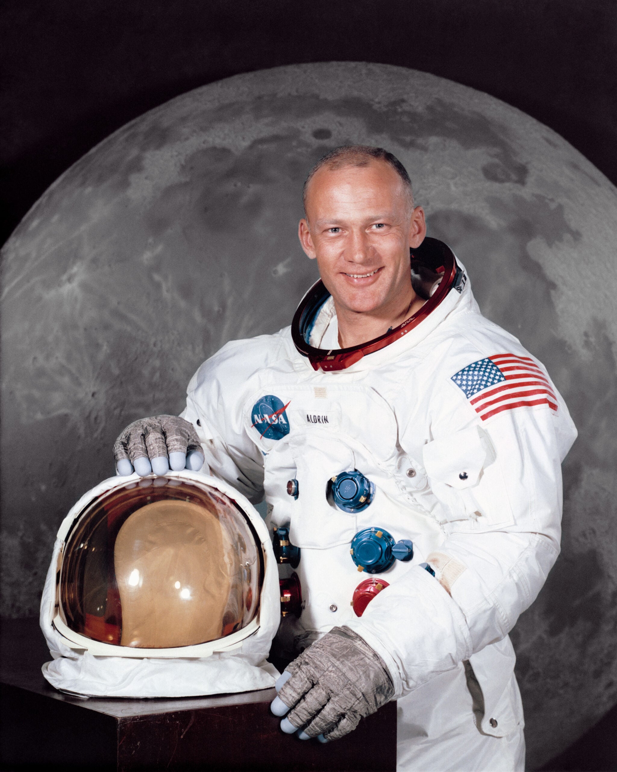
The second man to walk on the Moon later dug out his old expense claim from the trip, and it turns out Buzz Aldrin was reimbursed the grand sum of 33 dollars and 31 cents, not for the rocket or the spacecraft, but for the ordinary travel expenses of getting himself to and from the launch site like any other business trip.

The Apollo 11 mission cost NASA more than twenty billion dollars in 1969 money, or somewhere north of one hundred and fifty billion dollars in modern terms. It was one of the most expensive single scientific undertakings in human history, involving roughly four hundred thousand people across NASA and its contractor network. Everything about it was unprecedented. The Saturn V rocket had never been flown with a crew on a full lunar trajectory before. The Lunar Module had never been landed on a celestial body. The re-entry profile at the return end of the trip had never been survived. Buzz Aldrin flew on the mission as the second of three crew members and walked on the lunar surface on 20 July 1969. He returned home four days later. And when he got back to Houston he filed a routine federal government travel expense claim like any other public employee returning from a work trip. It was for thirty-three dollars and thirty-one cents.

What the voucher actually itemises

Aldrin posted a photograph of the original voucher on Twitter on 30 July 2015 to mark the forty-sixth anniversary of the moon landing. According to CBS News reporting the following day by science journalist Amanda Schupak, the voucher covers the period from 7 July 1969 through to 27 July 1969, which is a week and a half before the launch through to three days after the splashdown. What follows is probably the strangest business trip itinerary in the history of American federal expense accounting. The listed points of travel are Houston, Texas to Cape Kennedy, Florida on 7 July, then Cape Kennedy to Moon on 16 July, then Moon to Pacific Ocean on 24 July, then Pacific Ocean to Hawaii the same day, and finally Hawaii back to Houston on 27 July. The mode of transport listed for each leg is equally striking. Government Air for the two flights inside the continental United States. Government Spacecraft for the leg between Cape Kennedy and the Moon. USS Hornet, which is the aircraft carrier that recovered the crew, for the leg between the Pacific Ocean and Hawaii. And a US Air Force plane for the return to Houston.

The life of an astronaut is truly fascinating – check out the video we made on what every astronaut sees in the mirror:

The federal expense reimbursement system in 1969 did not distinguish between astronauts and any other government employee. If you were travelling on official business you filled out the same form, listed the same route, claimed the same mileage rate for personal vehicle use, and provided the same receipts for any out-of-pocket costs. Aldrin’s voucher was processed by a routine NASA finance office alongside vouchers from technicians attending conferences and administrators travelling to Washington. Nobody appears to have thought the situation odd enough to route it through any special channel. The reimbursement was paid in the normal course of business a few weeks later.

Why the amount was so small

The reason the total came to only thirty-three dollars and thirty-one cents rather than something more substantial is spelled out on the voucher itself. According to BBC Science Focus Magazine’s August 2015 write-up by Rachel Baxter, the document states in plain text that government meals and quarters were furnished for all the dates in question. That covered his food and lodging at the pre-launch quarantine facility at Cape Kennedy, aboard the Saturn V and the Apollo capsule, on the lunar surface itself, aboard the USS Hornet during the post-splashdown recovery, and inside the mobile quarantine facility where he and Neil Armstrong and Michael Collins were confined for twenty-one days after their return in case they had brought back any unknown lunar pathogens. The federal government had covered every one of those things directly, so Aldrin had nothing to claim against any of them.

What the thirty-three dollars and thirty-one cents actually covered was almost certainly the mileage rate for driving his own personal vehicle from his home in Houston to Ellington Air Force Base and back at each end of the trip. Government employees in 1969 were entitled to claim a per-mile rate when using their own car for official business. Aldrin did what everybody at NASA did. He drove to the airfield, got on the government plane, and came home the same way at the end. He submitted his mileage on the standard form. He got his check for thirty-three dollars and thirty-one cents in the mail a few weeks later.

The voucher was not the only piece of Apollo 11 bureaucratic paperwork Aldrin dug out and shared publicly in 2015. He also posted the US Customs declaration that he and Armstrong and Collins had signed on landing in Honolulu after the recovery. The declaration listed their country of departure as Moon and their flight number as Apollo 11. The cargo section listed moon rock and moon dust samples. The question about whether any crew member had been in contact with an infectious disease during the trip was answered by Aldrin in the space provided as “moon disease TBD.” A Honolulu customs inspector had counter-signed the form and accepted it as filed. The crew had cleared customs.

What the whole set of documents represents is one of the more revealing curiosities of the entire Apollo programme. NASA had achieved something in July 1969 that no human institution had ever previously come close to achieving, and the federal bureaucracy processing the paperwork for the people who had done it treated them exactly like every other federal employee returning from a work trip. That was partly because the routine forms were the only ones available. But it was also because the people at NASA didn’t consider themselves exempt from the ordinary paperwork obligations of federal employment. Aldrin filled out his expense form. He submitted his customs declaration. He collected his thirty-three dollars and thirty-one cents. And forty-six years later he still had the voucher in a drawer.

The post The second man to walk on the Moon later dug out his old expense claim from the trip, and it turns out Buzz Aldrin was reimbursed the grand sum of 33 dollars and 31 cents, not for the rocket or the spacecraft, but for the ordinary travel expenses of getting himself to and from the launch site like any other business trip. appeared first on Space Daily.

  •  

More than 2,500 retired New York subway cars were dropped into the Atlantic between 2001 and 2010, not as illegal dumping but as a planned reef programme, and marine biologists who kept watch found the sunken trains quickly turned into some of the richest artificial habitats along the eastern seaboard.

The Metropolitan Transportation Authority, which runs the New York City subway system, had a problem in the late 1990s. It was in the middle of a major fleet modernisation programme that was going to retire roughly two and a half thousand ageing subway cars over the following decade. These were mostly the red-painted R-33 and R-36 cars that generations of New Yorkers had ridden through the 1970s, 80s and 90s, followed by the older stainless steel Brightliners that would come off the tracks later. Each retired car was worth essentially nothing as scrap. Each also cost the MTA roughly twelve thousand dollars to dispose of through conventional demolition. Which meant the total disposal bill for the fleet retirement, at prevailing rates, was going to run to something north of thirty million dollars. And the MTA, being a public transit authority in a permanent state of budget crisis, was not enthusiastic about that particular expense.

The solution the agency arrived at, in partnership with a handful of coastal state governments and the U.S. Fish and Wildlife Service, was one of the more counterintuitive recycling programmes of the early twenty-first century. Instead of paying to demolish the cars, the MTA would clean them, ship them south by rail and barge, and drop them into the ocean off the eastern seaboard. There they would form artificial reefs. The states would get new marine habitat for essentially free. The MTA would save the disposal costs. And the fish would, in theory, work out what to do with the rest.

How you turn a subway car into a reef

According to the New York Transit Museum’s own summary of the MTA Artificial Reefing Program, produced in collaboration with the programme’s former director Michael Zacchea and Robert Martore of the South Carolina Department of Natural Resources, the operation ran from August 2001 through to April 2010 and deployed more than 2,500 deaccessioned train cars to underwater sites off the coasts of New Jersey, Delaware, Virginia, South Carolina, and Georgia. The first phase concentrated on the Redbird fleet, which was already being pulled off the tracks in 2001, and which had a particularly recognisable red livery that made the sunken cars a photographable subject long after they had gone down. The Delaware Bay took approximately six hundred and nineteen Redbird cars alone, at a site now known as the Redbird Reef, located sixteen and a half nautical miles off Indian River Inlet at a depth of around eighty feet. Subsequent phases involved the stainless steel Brightliner fleet, which was deployed at reef sites further down the coast through the second half of the decade.

The engineering of the actual reef deployment was not trivial. Each car had to be stripped down first. According to the New Jersey Division of Fish and Wildlife’s own news bulletin on the deployment of 44 stainless steel subway cars at the Atlantic City Reef site in April 2008, every car went through a full preparation process before it went into the water. Windows were removed. Wiring was pulled out. Plastic components, degradable materials, hydraulic fluids, oils, and grease were all stripped or drained. The remaining shell was inspected to make sure that when the car eventually corroded, nothing toxic would leach into the surrounding marine environment. Only after that inspection was the cleaned steel body loaded onto a barge and towed offshore.

The actual sinking process was almost comically straightforward. The cars, weighing around eighteen tonnes each in their prepared state, were rolled off the deck of the barge by a hydraulic tipping mechanism and simply dropped through the water column to the seabed below. The MTA covered all of the cleaning, transport, and deployment costs. Individual cars in the New Jersey deployment measured roughly sixty feet long, ten feet wide, and eleven feet tall. Deployed in tight clusters at pre-selected coordinates, they formed roughly the same kind of hard-structure habitat that a natural rocky reef would offer, but at a scale and geometry that had never previously existed on the sandy Atlantic continental shelf.

What the fish did with them

What happened next surprised the marine biologists monitoring the sites, though it probably shouldn’t have. The subway car reefs, unlike almost any natural feature of the mid-Atlantic seabed, offered vertical structure. They offered cavities and shelter. They offered hard surfaces for sessile organisms to colonise. And they were essentially unlimited in supply. Marine invertebrates began settling on the exposed steel within weeks. Barnacles arrived. Blue mussels followed. Sponges and soft corals began to establish themselves on the vertical surfaces. Within a year or two, the once-bare metal shells of the retired subway cars had become the physical scaffolding of thriving benthic communities that had not existed anywhere on that stretch of ocean floor beforehand.

The fish arrived in response. Delaware’s Department of Natural Resources and Environmental Control has since documented that the invertebrate communities colonising the artificial reef structures provide up to four hundred times more food per square foot than the bare sandy ocean floor they replaced. Species that had been effectively absent from the region because of the lack of suitable habitat began to appear regularly at the sites. Sea bass, tautog, tuna, mackerel, flounder, scup, and triggerfish were all documented in significant numbers within a few years of the deployments. Recreational fishing operators in the coastal towns of Delaware, New Jersey, and Virginia found their nearshore catches rising. Dive operators found themselves with a genuinely unusual attraction to offer. The sunken subway cars, which had cost the MTA nothing to dispose of and had cost the states essentially nothing to acquire, became one of the more productive artificial reef complexes anywhere on the North American Atlantic coast.

The programme was not without complications. Inspection reports from New Jersey in 2009 found that some of the newer stainless steel subway cars were showing significant structural damage after only a few years underwater, which prompted the state to pause further stainless steel deployments while investigations continued. Not every car remained intact. Not every deployment site delivered the ecological returns the biologists had hoped for. And the specific question of whether artificial reefs simply concentrate existing fish populations rather than creating new ones is still debated within the marine biology community. But the general pattern held across the majority of the deployment sites through the 2010s and 2020s. The bare sand became structured habitat. The structured habitat became invertebrate communities. The invertebrate communities became feeding grounds. And the feeding grounds became fisheries.

By the time the programme officially ended on Earth Day 2010, 2,580 New York subway cars had been placed on ocean reef sites along the eastern seaboard of the United States. The MTA had saved something close to thirty million dollars in disposal costs. Delaware alone had received nearly a thousand of them. The Redbird Reef off Slaughter Beach now covers roughly 1.3 square miles of what used to be featureless sand and is one of the most biologically productive stretches of continental shelf in the entire mid-Atlantic region. Which is a strange kind of legacy for a fleet of subway trains that once carried millions of people through the tunnels underneath Manhattan and Queens. The trains never made it to the recycling yard. They made it to the ocean floor instead. And the fish have been living in them ever since.

The post More than 2,500 retired New York subway cars were dropped into the Atlantic between 2001 and 2010, not as illegal dumping but as a planned reef programme, and marine biologists who kept watch found the sunken trains quickly turned into some of the richest artificial habitats along the eastern seaboard. appeared first on Space Daily.

  •  

Four fixed half-pipe reflectors in British Columbia, each 100 meters long and strung with 1,024 antennas, watched the same overhead strip of sky from July 25, 2018 to September 15, 2023 and logged 4,539 fast radio bursts from 3,641 separate sources, on a telescope that cannot be aimed.

A telescope with no moving parts, stationed in the mountains of British Columbia, has produced the largest single accounting of fast radio bursts ever assembled. The Canadian Hydrogen Intensity Mapping Experiment (CHIME) and its FRB collaboration have released a second catalog logging 4,539 fast radio bursts from 3,641 distinct sources, drawn from more than five years of continuous sky-watching between July 25, 2018, and September 15, 2023.

The result, posted to arXiv in January 2026 and published in The Astrophysical Journal Supplement Series, supersedes the collaboration’s first catalog, which covered a single year of observations ending in mid-2019 and recorded 536 bursts. The new release spans roughly five times the observing period and delivers more than eight times as many detected events, cementing CHIME’s role as the dominant instrument for cataloging these millisecond-long flashes of radio energy.

A telescope that cannot look anywhere else

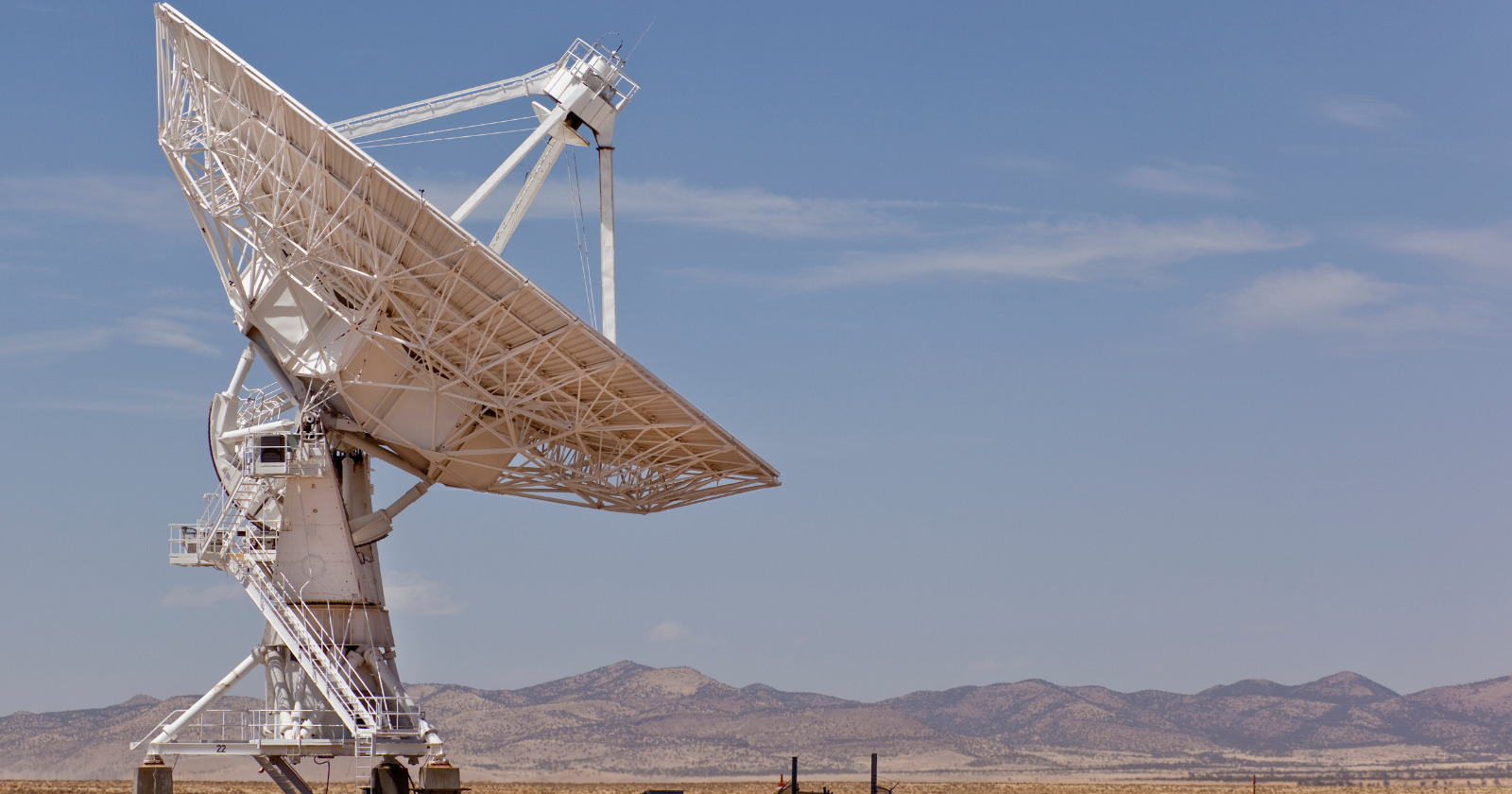
CHIME’s design is unusual for an instrument that has become the world’s leading fast radio burst detector. Located at the Dominion Radio Astrophysical Observatory near Penticton, British Columbia, it consists of four stationary half-pipe reflectors, each 100 meters long and 20 meters wide, laid side by side and oriented north-south. ICHIME has no moving parts at all — unlike dishes that swivel to track a target. Each cylinder’s focal line is strung with 256 dual-polarization antennas, for 1,024 across the array, feeding a digital signal-processing system that forms 1,024 beams electronically rather than through any physical steering.

That fixed geometry means CHIME cannot be aimed at a particular patch of sky the way a conventional radio dish can. Instead, it watches a roughly 200-square-degree strip of sky directly overhead and lets Earth’s rotation carry the rest of the northern sky through its field of view over the course of a day. The technique, known as transit observing, trades the ability to target specific objects on demand for near-continuous coverage of a wide swath of sky, night and day — precisely the kind of monitoring that catching rare, unpredictable millisecond bursts requires.

What changed since the first catalog

The collaboration’s first catalog, released in 2021, logged just over 500 bursts from a single year of data. That release established CHIME as a serious FRB survey instrument and provided the first large, uniformly selected sample for statistical study. The new catalog is a different scale of effort entirely: it folds in more than four additional years of observing time, past the original one-year window, and pushes the source count past 3,600 — a population increase that lets researchers move from spotting a phenomenon to characterizing it as a class.

Fast radio bursts are intense pulses of radio waves lasting typically a few milliseconds, first identified in archival data in 2007 and confirmed as an astrophysical population in the years since. Most detected bursts appear to flash once and never repeat from the same location, but a minority repeat, sometimes many times, from sources that can be pinpointed to host galaxies. Among the 4,539 bursts in the new catalog, 981 come from 83 known repeating sources, while the remainder appear as one-off events, at least within the observing window. That repeater fraction, drawn from a sample nearly nine times larger than before, gives researchers a substantially firmer basis for comparing the properties of repeating and apparently non-repeating bursts, including their durations, frequency structure, and the dispersion imposed on the signal as it crosses intervening plasma on its way to Earth.

Why the larger sample matters

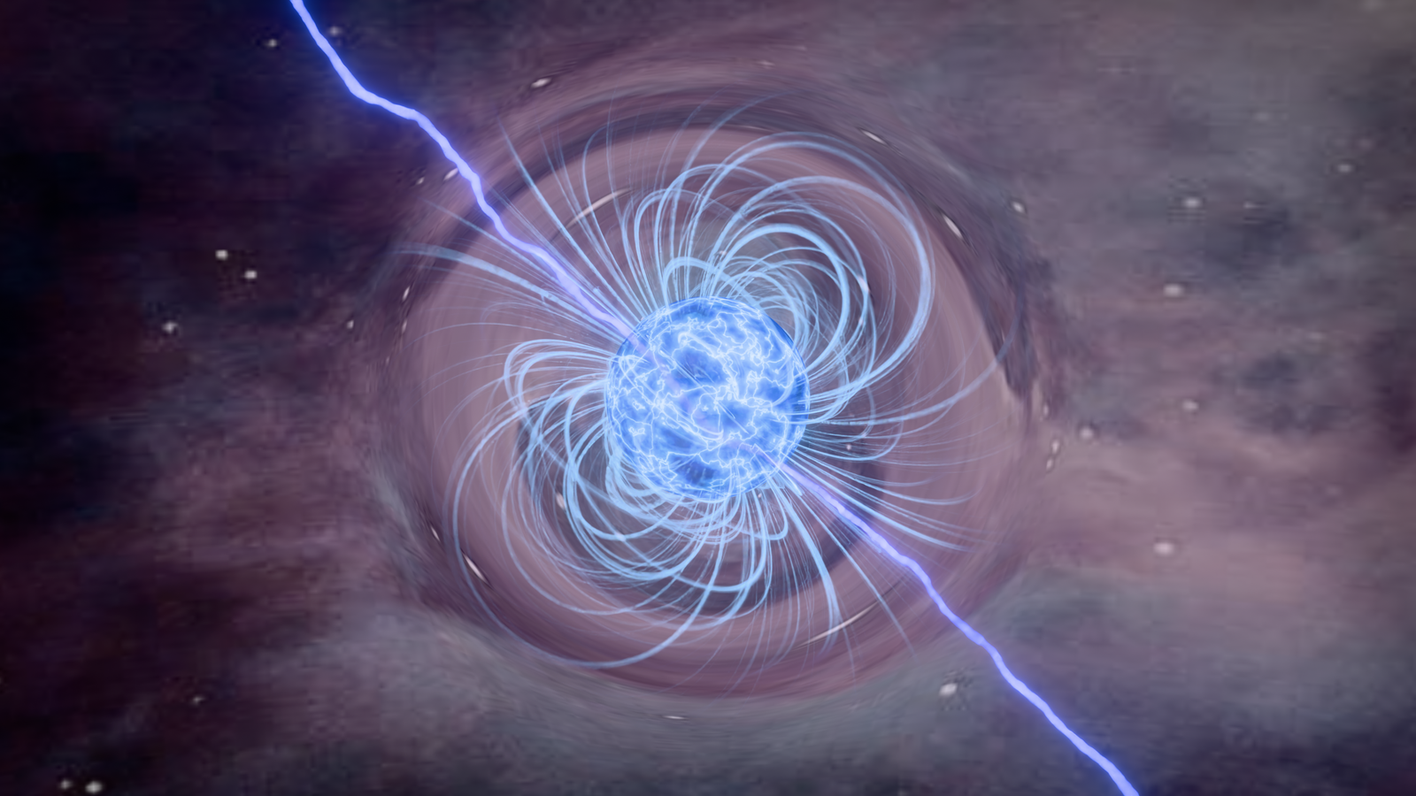
The physical origin of fast radio bursts remains only partly settled. Magnetars — neutron stars with extraordinarily strong magnetic fields — are the leading candidate source for at least some bursts, following the 2020 detection of a burst from a magnetar inside the Milky Way. But the diversity of burst durations, brightness, and repetition behavior recorded across thousands of events suggests more than one physical mechanism, or more than one class of source, may be responsible. Larger, more uniform catalogs let researchers test that diversity statistically rather than relying on a handful of well-studied individual sources.

Because each burst’s radio signal is dispersed — delayed by different amounts at different frequencies as it passes through free electrons in space — the catalog also functions as a probe of matter distributed between galaxies. That diffuse, low-density gas is difficult to detect by any other means, and a sample of thousands of bursts at known or estimated distances allows astronomers to map its distribution across large volumes of the universe, an application sometimes described as using fast radio bursts to weigh the cosmos.

The catalog paper reports each burst’s arrival time, dispersion measure, scattering timescale, and flux density, along with a dynamic spectrum across the 400–800 megahertz band CHIME observes, at just under a millisecond time resolution. That level of detail, applied uniformly across thousands of bursts rather than compiled from disparate instruments and detection methods, is what distinguishes a catalog release from a series of individual discovery announcements.

What comes next

CHIME/FRB’s outrigger stations — companion antenna arrays built at separate sites across North America — extend the core telescope’s ability to localize individual bursts to their host galaxies with far greater precision than CHIME alone can achieve, a capability that has already been applied to a subset of local-universe bursts drawn from the same multi-year dataset. As those outriggers accumulate their own detections alongside the main array, the size and precision of future catalogs are expected to grow further, sharpening the statistical picture the second catalog has already begun to draw.

The post Four fixed half-pipe reflectors in British Columbia, each 100 meters long and strung with 1,024 antennas, watched the same overhead strip of sky from July 25, 2018 to September 15, 2023 and logged 4,539 fast radio bursts from 3,641 separate sources, on a telescope that cannot be aimed. appeared first on Space Daily.
  •  

Physicist Bhupal Dev at Washington University used the debris from GW170817 — the 2017 neutron star merger — to squeeze new limits on axion-like particles, treating the hot post-collision remnant as a natural forge for dark-matter candidates

Physicist Bhupal Dev at Washington University used the debris from GW170817 — the 2017 neutron star merger — to squeeze new limits on axion-like particles, treating the hot post-collision remnant as a natural forge for dark-matter candidates

For about one second after two neutron stars collided 130 million light-years away, the wreckage they left behind was hotter than anything else in the observable universe. Bhupal Dev, a physicist at Washington University in St. Louis, and four collaborators asked what that one second would have manufactured if a hypothetical particle called an axion-like particle exists — and then went looking for the light it should have left behind.

Nothing arrived. The shape of that absence is the result.

What GW170817 actually was

On 17 August 2017, the LIGO and Virgo detectors recorded a gravitational-wave chirp lasting roughly 100 seconds, the longest signal captured to that point. About 1.7 seconds later, NASA’s Fermi Gamma-ray Burst Monitor caught a short gamma-ray burst from the same patch of sky. The coincidence is documented in the collaboration’s multi-messenger paper in The Astrophysical Journal Letters.

Less than eleven hours after the merger, the one-metre Swope Telescope in Chile pinned the source to NGC 4993, a lenticular galaxy about 40 megaparsecs — roughly 130 million light-years — away. Within a day, dozens of observatories were watching a fading point of light that astronomers had spent decades predicting and never seen: a kilonova.

Two neutron stars had spiralled into each other, each somewhere between about one and two times the mass of the Sun, each compressed into an object about the size of a mid-sized city. When they touched, the collision briefly produced conditions denser and hotter than anywhere else in the observable universe.

neutron star merger illustration

ESO’s telescopes in Chile tracked the afterglow across a wide range of wavelengths, and the observatory’s October 2017 announcement of the first visible counterpart to a gravitational-wave source reported spectra suggesting caesium and tellurium in the ejecta. Two years later, a separate analysis of VLT X-shooter data pinned down strontium, the first individual heavy element identified in a neutron star collision. Some of the gold in a wedding ring was made in events like this one.

Why the remnant is a particle factory

Before they merge, neutron stars are cold by particle-physics standards — thermal energies around a kilo-electron-volt. The collision changes that within milliseconds. Temperatures in the remnant climb into the tens of MeV, and the benchmark merger profile Dev’s group used exceeds 50 MeV in places, roughly 600 billion degrees. Production rates for weakly coupled particles rise steeply with temperature. Whatever exists in the right mass window gets made.

Axion-like particles, or ALPs, are among the most-hunted candidates. They are cousins of the axion — the particle implied by the Peccei-Quinn mechanism proposed in 1977 to resolve a puzzle in the strong nuclear force, and named the following year by Weinberg and Wilczek. ALPs relax the axion’s strict relationship between mass and coupling, and they appear generically in string theory and in many extensions of the standard model.

The catch is that they interact with ordinary matter so feebly that laboratory experiments struggle to reach the parameter space that matters. Which is where dead stars come in.

How the bound actually works

The property Dev’s group targeted is the ALP’s coupling to photons. In the hot, dense matter of the remnant, two processes make ALPs: the Primakoff process, in which a photon scattering off a proton converts into an ALP, and photon coalescence, in which two photons merge into one. Primakoff dominates at low masses, coalescence at high ones, with the switchover around 100 MeV.

What happens next is the whole argument. ALPs stream out of the remnant — those with enough kinetic energy to climb out of its gravitational well, at least — and then decay back into pairs of photons well outside the debris. The team required decays beyond about 1,000 kilometres, far enough that the emitted photons would not simply be reabsorbed by the ejecta. The result would be a gamma-ray signal arriving roughly along the line of sight to the merger, offset in time from the gravitational waves by the geometry of where each ALP happened to decay.

Fermi-LAT was watching. It missed the prompt burst, but it collected data in the window from 1,153 to 2,027 seconds after the gravitational-wave signal, across 0.1 to 1 GeV, and saw nothing above a flux upper limit of 4.5 × 10⁻¹⁰ erg per square centimetre per second at 95% confidence. Every combination of ALP mass and photon coupling that would have produced a brighter signal than that is excluded. The preprint sets out the full calculation, including the decay geometry and the in-medium photon physics.

That is the first constraint of its kind derived from a merger, as the university’s announcement of the work noted. Two representative points in the newly excluded region sit at masses of 200 and 398 MeV. Worth being precise about what this is not: it is not a cooling argument. The team explicitly checked that across the parameter space they constrain, ALP emission does not drain enough energy to alter how the remnant cooled.

What the bound covers, and what it does not

The GW170817 exclusion is weaker than the long-standing limit from Supernova 1987A, and the reason is geometry rather than physics. Photon flux at Earth falls off with the square of the distance to the source. A supernova in the Large Magellanic Cloud is far closer than a merger at 40 megaparsecs, so it delivers more photons even from an identical ALP population.

What the merger offers instead is timing. The arrival of the gravitational-wave signal defines a clean zero point, which supernovae generally lack — for SN 2023ixf, no neutrino signal was detected at all. Combining spectral and temporal information from a merger, the authors argue, is where this method becomes competitive, particularly for observations inside the first second.

The constraint is also more robust than the article’s underlying uncertainties might suggest. GW170817’s remnant is thought to have survived about a second before collapsing to a black hole; varying that assumed lifetime between 0.72 and 1.29 seconds barely moves the exclusion region, and the result depends only weakly on which of nine merger profiles is used.

None of this detects anything. It tells you what an ALP cannot be, given that GW170817 behaved the way it did. And the dark matter question is separate again: an ALP in this mass range could in principle be a dark matter component, but a production bound from one merger says nothing about cosmological abundance. It shrinks the box. It does not confirm anything is in it.

The source that keeps giving

The merger’s own story has kept moving independently of the particle physics. Chandra saw nothing when it first slewed to the target, then found a point source on 26 August 2017. That sequence — non-detection, then detection — was itself the clue. It indicated a narrow relativistic jet pointed away from Earth, whose emission only reached the detector once the jet slowed and widened into the line of sight.

Chandra X-ray observatory

Then the fading stopped. As the Center for Astrophysics reported in March 2022, Aprajita Hajela of Northwestern University and colleagues found that from March 2020 through the end of that year the X-ray brightness held roughly constant. Something besides the jet had taken over. The two candidates are a kilonova afterglow — a shock from the expanding debris — or matter falling onto a newly formed black hole. Either would be a first, and radio observations are the test: a kilonova afterglow should brighten in radio, accretion onto a black hole should not.

At the time of that release, Chandra was the only observatory still able to detect the source, more than four years after the collision.

Space Daily has covered other corners of the same search. A Rice University team has used a grain-of-sand-sized magnet levitated above a superconductor to hunt for ultraheavy dark matter, extending the search toward candidates approaching the mass of a living cell, according to the group’s own account of the experiment. That is the far end of the mass axis from the MeV-scale ALPs Dev’s group is bounding — a table-top instrument at millikelvin temperatures on one side, a collision 130 million light-years away on the other.

Using distant catastrophes as instruments

GW170817 remains the only confirmed binary neutron star merger with a full electromagnetic counterpart. LIGO and Virgo have caught other candidate neutron star events, but none produced the same multi-wavelength bounty, which is why the same dataset keeps being reprocessed for new physics. A 2021 review by Milton Ruiz, Stuart Shapiro and Antonios Tsokaros in Frontiers in Astronomy and Space Sciences surveys what relativistic simulations can now say about these events, including the consensus that GW170817’s remnant lasted under a second before collapsing.

A cleaner ALP constraint needs more mergers, or closer ones. The authors sketch both: a stacked analysis of several events, a hypothetical merger ten times nearer, and early observation windows starting a tenth of a second after the gravitational-wave trigger. Proposed MeV gamma-ray missions such as AMEGO-X and e-ASTROGAM would help considerably.

When that data arrives is unsettled. O4 ended on 18 November 2025, and the detectors have since been in upgrades and commissioning. According to the LIGO-Virgo-KAGRA observing plan, an interim six-month run is expected around late 2026, while the timeline for the fifth observing run remains under discussion.

The hot phase of the merger lasted about one second. The gravitational-wave chirp lasted about a hundred. Somewhere between those two numbers is a photon signal that never reached Fermi’s detectors — and the precise shape of that absence, how bright it wasn’t and how early it wasn’t, is what now fences off a corner of parameter space where a particle nobody has ever seen can no longer hide.

The post Physicist Bhupal Dev at Washington University used the debris from GW170817 — the 2017 neutron star merger — to squeeze new limits on axion-like particles, treating the hot post-collision remnant as a natural forge for dark-matter candidates appeared first on Space Daily.
  •  

On 28 October 1971, a British Black Arrow rocket put Prospero into orbit from the Australian desert — Parliament had been told on 29 July that the programme would end after this flight, leaving the next rocket to become an unflown museum exhibit.

A red dirt road stretching across a flat Australian outback landscape

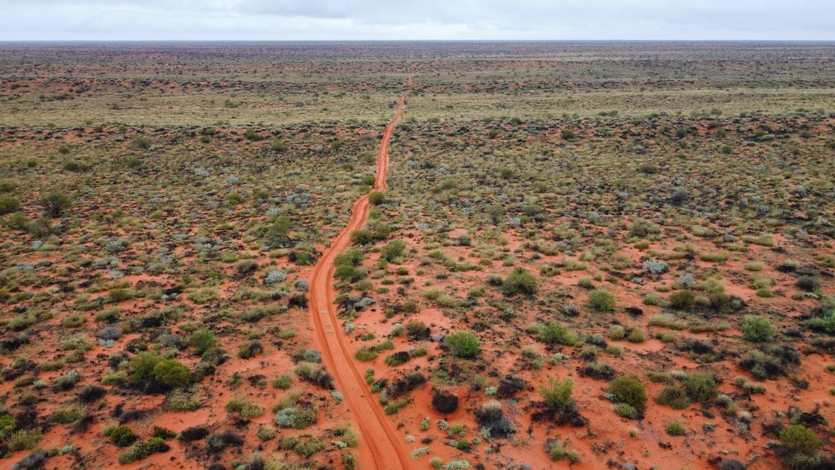
Black Arrow’s successful orbital flight arrived after its future had already been decided. On 28 October 1971, the British rocket launched Prospero from Woomera, Australia. Three months earlier, Parliament had been told that the programme would end once that mission was complete.

The next vehicle, R4, never launched. Its eventual place in the Science Museum gives the story a physical ending: one rocket carried a satellite into orbit, while its successor became an object through which later generations could examine the programme.

The final flight was explicitly allowed

The written parliamentary answer of 29 July 1971 is unusually clear. Responding to a question about the National Space Technology Programme, Frederick Corfield confirmed plans to launch the X3 satellite later that year. He then stated that Black Arrow would be terminated after the launch.

That matters because it distinguishes an authorised final mission from a launch carried out in defiance of cancellation. The decision and the permission appeared in the same answer. The engineers could complete the flight, but a successful result was not accompanied by a promise of further launches.

Corfield’s stated rationale concerned resources and capability. Maintaining a national launcher with comparatively limited capacity, he argued, consumed too much of the available programme while restricting its broader scope. The answer also said satellite technology research would continue, with X4 planned for a NASA Scout launch in 1974.

The launcher was ending; satellite work was continuing.

A British vehicle launched from Australia

ESA’s historical account confirms the date, the Woomera launch site and Prospero’s alternative designation, X3. Black Arrow’s development had begun in 1964 under the Royal Aircraft Establishment. Its achievement was the delivery of a satellite by a British-developed launcher, not a launch from British soil.

That distinction is easy to lose in a compressed account of national space achievements. The origin of a rocket, the origin of its payload and the territory from which it flies are separate facts. Here, the Australian desert was part of the infrastructure that made the British programme possible.

A UK Space Agency retrospective describes the wider effort behind the vehicle: rocket and engine development, assembly and test facilities in Britain, and launch and range facilities at Woomera. Black Arrow drew on earlier Royal Aircraft Establishment research and technologies using high-test peroxide and kerosene.

The agency describes a three-stage rocket about thirteen metres tall, with an eight-chamber engine in the first stage and a solid motor in the third. Those modest dimensions can obscure the range of systems required to produce an orbital flight. A launch vehicle is also a programme of testing, ground support, control and integration.

R4 records the launch that did not happen

The Science Museum Group’s collection record for Black Arrow R4 identifies it as the final vehicle built, with minor assembly and pipework incomplete. Its intended satellite, Miranda, eventually went into orbit on an American Scout rocket in 1974.

R4 is therefore more than a representation of the rocket that flew. It is surviving hardware from the next step that the programme did not take. Its parts preserve engineering decisions even though they never experienced a launch.

The museum records four Black Arrow launches, two successful, including the flight that orbited Prospero. That is a short development history, and it invites competing readings: a capability achieved just as support ended, or a limited programme whose costs had to be weighed against other space priorities.

The records establish the sequence without settling every argument about the decision. A successful flight demonstrates that a particular mission worked. It does not, on its own, calculate the costs, demand or reliability of an extended operational service. Equally, a decision to stop funding that service does not undo the technical achievement.

Becoming an exhibit required another decision

A Science Museum Group Journal study of R4 follows the vehicle’s transition into a museum object. It describes discussions soon after Prospero’s launch, when the departments responsible for Black Arrow were working towards winding up the programme by the end of March 1972.

Acquiring the rocket involved practical arrangements, not simply declaring it historic. The article records an estimated £5,000 to prepare it for transfer, to be met by the Department of Trade and Industry, with the museum responsible for transport from the Isle of Wight to its west London store.

The preservation of a cancelled project is itself work. Large objects need space, handling equipment and decisions about what to retain. Without those choices, the next rocket might have survived only in drawings and photographs.

R4 became evidence that people could stand beside.

Success and continuation were different questions

Black Arrow’s ending is often compelling because the chronology seems reversed: the programme was told to stop, then achieved its orbital goal. But the parliamentary statement shows that both outcomes had already been accommodated. The final flight could proceed while the longer-term launcher commitment ended.

Space Daily’s account of Project West Ford’s orbiting copper needles describes another space experiment whose technical demonstration did not lead to an enduring operational system. The reasons differed, but both histories reward separating what hardware proved from what institutions chose to continue.

Prospero’s launch and R4’s preservation mark those two questions in different places. One was answered above the Australian desert in October 1971. The other left a rocket on Earth, retaining the shape of a next flight that never came.

The post On 28 October 1971, a British Black Arrow rocket put Prospero into orbit from the Australian desert — Parliament had been told on 29 July that the programme would end after this flight, leaving the next rocket to become an unflown museum exhibit. appeared first on Space Daily.

  •  

Cambridge researchers kept a computer chip running for a year using blue-green algae in a container about the size of an AA battery — the living power source harvested energy from light and continued supplying electricity through periods of darkness

A tube of pond scum on a Cambridge windowsill spent half a year running a computer, and nobody had to feed it.

The container held blue-green algae, water and very little else, and it was roughly the size of an AA battery. Inside it, a colony of microbes harvested light, leaked electrons into a strip of aluminium and produced a current steady enough to keep a microprocessor ticking over from February to August 2021. Smithsonian magazine reported that the whole apparatus sat out a pandemic lockdown on a windowsill in the home of Cambridge biochemist Paolo Bombelli.

It ran far longer than anyone on the project expected.

What was actually inside the container

Synechocystis is a cyanobacterium, one of the ordinary non-toxic pond dwellers that has been quietly photosynthesising for a couple of billion years. Photosynthesis splits water and sends the resulting electrons down an internal transport chain inside the cell. Some of that current leaks out before it is used, and a metal anode positioned nearby can catch it. Exactly how those electrons make the jump from a living cell to bare metal is still not settled.

Bombelli and his colleagues, writing in Energy & Environmental Science, described a small housing of clear plastic and steel with an aluminium anode inside, built from inexpensive and largely recyclable parts. No feeding, no charging. Cyanobacteria make their own food as they photosynthesise, so light and water cover the entire supply chain.

Stranger still, the current did not stop at sunset. Researchers on the team suspect the microbes carry on metabolising food banked earlier in the day, which is why the cell kept nudging out electricity through the dark hours, as the Cambridge Independent reported.

How little electricity this really is

Averaged across the experiment, the cell delivered about 1.05 microwatts at 0.72 volts, figures Gizmodo set against the obvious comparisons. A fresh AA battery starts life at 1.5 volts. An efficient LED globe pulls around 10 watts. So the device was generating something in the region of a ten-millionth of a globe.

That sufficed only because the chip had been picked for extreme frugality. An Arm Cortex M0+ can tick along on 0.3 microwatts, and Arm Research built the test chip, the board and the cloud link that logged everything the microbes did. Only the chip itself ran on that current. The cloud link, which reported the results back to the researchers, needed conventional power to do its job.

Devices of this kind hold one advantage over the better-known microbial fuel cell, which needs a steady diet of organic matter to keep its bacteria working. Researchers publishing in Nature Communications noted that biophotovoltaic systems skip that input altogether, since the cells feed themselves as they go. The fuel bill is nothing and the colony renews itself, roughly the combination a sensor buried in a paddock for a decade would want.

Why a microwatt earns a paper

Who needs a computer powered by pond water? Nobody, right now. The argument is about the enormous, boring category of devices that comes next: door sensors, soil monitors, tracking tags, all the small gadgets multiplying across the world. Forecasts in the same paper put the number of connected devices on a path towards a trillion by 2035, every one of them wanting its own portable trickle of electricity. Batteries go flat, and they depend on materials that are expensive and unpleasant to dig out of the ground.

Christopher Howe, the Cambridge biochemist who co-led the work, argued in the university’s announcement that supplying all that hardware will require systems that generate energy “rather than simply store it like batteries”.

What one windowsill proves

Six months of unbroken output went into the submitted paper, and the hardware simply carried on afterwards. The funders at the National Biofilms Innovation Centre later described the microprocessor as having run for a year and counting on nothing but ambient light and water.

A single device in a single house is a demonstration, and one paper is one paper.

Two things stand between this and anything resembling a product: a great deal more current, and some agreement on how to measure it. A review in Frontiers in Microbiology characterises biophotovoltaics as a field hobbled by very low current outputs and by experimental set-ups too inconsistent to compare with each other, which stalls any systematic push to improve them. No one has fully pinned down how electrons cross from a living cell into an electrode either, so progress tends to come from trying things and seeing what sticks.

Scaling up means manufacturing thousands of these cells cheaply and reliably, and doing it before anyone has fully worked out what is happening inside them.

The processor was disconnected a long time ago. By Bombelli’s account the algae carried on making electricity regardless, entirely indifferent to whether anything was still listening.

The post Cambridge researchers kept a computer chip running for a year using blue-green algae in a container about the size of an AA battery — the living power source harvested energy from light and continued supplying electricity through periods of darkness appeared first on Space Daily.
  •  

French, Russian, and German researchers thawed sediment from nine sites of Siberian and Kamchatkan permafrost and revived thirteen previously undescribed viruses, the oldest of them from ground beneath a Yakutian lake bed dated to more than 48,500 years, and the reason every one of the thirteen can infect nothing but amoebae is a decision the team made before the first sample went into the dish

Thirteen viruses that have not circulated on Earth since before the last Ice Age’s coldest stretch are now, technically, alive again. A team led by Jean-Michel Claverie and Chantal Abergel at Aix-Marseille University, working with Russian colleagues from the Melnikov Permafrost Institute and other institutions, and German permafrost scientists from the Alfred Wegener Institute, pulled the samples from nine locations across Siberian and Kamchatkan permafrost and coaxed the ancient particles back into active replication in a lab dish. The oldest, a giant virus the team named Pandoravirus yedoma, came from sediment more than 16 meters beneath a thermokarst lake at Yukechi Alas in central Yakutia, radiocarbon-dated to over 48,500 years old. The strange part is not any of that. It’s that every single one of the thirteen, across five separate viral families, turned out capable of infecting exactly one thing: amoebae.

That is not a coincidence or a discovery about what these viruses are inherently limited to — it’s the result of a rule the researchers built into their methods before they ever opened a sample.

Nine sites, one very old lake bed, and a five-family haul

The study, published in the journal Viruses in February 2023, describes sampling seven ancient Siberian permafrost cores, a Lena River sediment sample, and one modern surface soil sample from Kamchatka as a comparison point. Out of that set, the team isolated 13 new viral strains spanning five clades: pandoraviruses, cedratviruses, megaviruses, pacmanviruses, and a new strain of pithovirus, the family first revived by the same lab back in 2014. Beyond the 48,500-year Pandoravirus yedoma strain, other samples dated to more than 27,000 and 28,600 years old, meaning the youngest viruses in the batch had still been dormant since well before agriculture existed anywhere on the planet.

Getting a virus that old to replicate again sounds harder than it is, mechanically. Permafrost is an unusually good preservative: constant sub-zero temperatures, no light, and low oxygen slow decay to something close to a standstill. The genuine difficulty was deciding what, exactly, the revived particles should be allowed to infect — not reviving them in the first place.

Why the answer was decided in advance

Every one of the 13 viruses was isolated using a single host organism: Acanthamoeba castellanii, a free-living amoeba common in soil and freshwater that happens to be an excellent, and epidemiologically inert, lab culture system for giant viruses. The paper’s own framing makes clear this was the point, not an accident: as the authors put it, the viruses recovered “belong to five different clades infecting Acanthamoeba spp.” precisely because of “the host specificity imposed by our protocol.” In plain terms, the team only exposed each sample to amoeba cultures, so the only viruses that could be detected at all were ones already capable of infecting amoebae. Anything in the sediment that might have targeted a mammal, a bird, or a human cell simply had no host present to reveal itself.

Claverie has been explicit about why that constraint exists. “Our protocol is to put amoeba cultures in the lab in contact with various samples, in the hope that they will contain viruses capable of infecting amoebas,” he told Live Science, adding a flatter, more direct version of the same point: “We will never risk isolating a virus eventually capable of infecting modern mammals.” The paper itself makes the comparison explicit, noting that the biohazard from reviving amoeba-only viruses is “totally negligible” next to the far riskier work of hunting for pathogens directly inside the frozen remains of mammoths and other ancient mammals, which is why that specific line of research is confined to a biosafety level 4 facility in Novosibirsk rather than an ordinary university lab.

Every choice the team made before opening a single sample was a choice about what they were willing to risk being wrong about.

The part that actually worries the researchers

That caution isn’t really about this batch of 13 viruses. It’s about what else permafrost is holding, and how much more of it is on its way to thawing. Claverie has made this argument before: back in late 2022, months before Pandoravirus yedoma’s record-setting age was even published, he told Newsweek, “If amoeba viruses can survive in these conditions, there is no reason for other viruses not to survive as well” — the same underlying logic the yedoma finding would go on to reinforce.

The paper’s own conclusion frames the risk in terms of exposure rather than certainty: nobody can currently estimate how long a thawed ancient virus would stay infectious once it hit open air, or how likely it would be to encounter a suitable host in that window. What has changed, and what makes the question worth asking at all, is the denominator. Arctic permafrost is thawing faster as the region warms, and industrial development, mining, and new settlements are sending more people into exactly the areas where 48,500-year-old ground is being exposed for the first time since before modern humans reached most of the planet. The amoebae were never really the point. They were the deliberately narrow lens the researchers chose so that the first question, can something this old still replicate at all, could be answered without opening a second, much harder question before anyone was ready to.

The post French, Russian, and German researchers thawed sediment from nine sites of Siberian and Kamchatkan permafrost and revived thirteen previously undescribed viruses, the oldest of them from ground beneath a Yakutian lake bed dated to more than 48,500 years, and the reason every one of the thirteen can infect nothing but amoebae is a decision the team made before the first sample went into the dish appeared first on Space Daily.

  •  

SpaceX has asked to operate up to one million AI satellites, but their direct waste heat would barely affect global temperature; the larger climate question is what launches and mass re-entry would put into the upper atmosphere

Representative rocket lifting off through a plume of exhaust

SpaceX has formally asked US regulators for permission to operate as many as one million AI data-center satellites. That number is real. It is also an upper limit in an application, not an approved fleet, a launch schedule or evidence that one million spacecraft will actually be built.

If the full Starmind system ever existed, its direct waste heat would be too small to become a major global climate driver. The harder environmental question lies in the industrial cycle required to create and replace it: manufacturing enormous amounts of hardware, launching it through the atmosphere and eventually vaporizing much of it during re-entry.

Climate models have only begun to study satellite constellations measured in tens of thousands. A million large computing satellites would sit far beyond the scale directly tested in that literature.

The FCC has accepted an application, not approved a million launches

SpaceX filed its application on January 30, 2026. The Federal Communications Commission accepted it for public comment on February 4.

The filing seeks authority for a non-geostationary system of up to one million satellites between 500 and 2,000 kilometers altitude. The spacecraft would exchange data through optical links and connect with SpaceX’s Starlink network.

Accepting an application for filing is an administrative step. It does not mean the FCC has determined that the architecture is safe, environmentally acceptable or technically achievable. The public notice also says SpaceX plans different hardware versions across multiple orbital shells, so “one million satellites” does not describe one fixed design.

SpaceX has since presented its first AI1 design for the Starmind system. The company’s published specifications give it a 120-kilowatt average compute load, a 150-kilowatt peak and a deployed wingspan of 70 meters.

The computers’ direct heat is not the main climate problem

Computers turn almost all the electricity they use into heat. In orbit, that heat cannot leave through air or cooling water because neither is available. Large radiator surfaces must emit it as infrared radiation.

One million AI1 satellites operating at the advertised average would use about 120 gigawatts for computing. To put a strict upper bound on the direct climate effect, imagine that every watt of that heat somehow reached and was absorbed by Earth. Spread over the planet’s surface, it would average roughly 0.00024 watts per square meter.

That artificial scenario overstates the real effect because radiators can direct most thermal radiation toward deep space. Even so, its value is more than 10,000 times smaller than the IPCC’s estimate of 2.72 watts per square meter for total human-caused effective radiative forcing between 1750 and 2019.

The fleet would therefore not warm Earth simply by running hot computers overhead. Reflected sunlight, radiator orientation and the design of vast solar arrays would still need assessment, but direct compute heat is not the dominant global term.

Space solar power could avoid some terrestrial emissions

SpaceX argues that sun-synchronous satellites could collect solar energy without clouds or night-time interruptions and reject heat without chillers, cooling towers or fans. If orbital computing genuinely replaced electricity from fossil-fueled grids, it could avoid some power-sector carbon emissions and water consumption.

That benefit cannot be calculated from the one-million figure. A fair comparison would need the energy and materials used to manufacture satellites and rockets, propellant production, launch emissions, ground stations, replacement rates, failed spacecraft and the carbon intensity of the terrestrial data centers displaced.

No published life-cycle assessment yet covers SpaceX’s proposed full system. “Powered by solar energy” describes operation in orbit, not the environmental balance of building and continually replenishing the fleet.

Rocket exhaust is unusually effective high in the atmosphere

Rocket emissions are small beside global aviation, shipping or power generation by mass. Their location makes them different. Rockets inject black carbon, water vapor, nitrogen compounds, alumina and other products directly into atmospheric layers that surface pollution rarely reaches.

Black carbon absorbs sunlight and warms the surrounding stratosphere, changing atmospheric circulation and ozone chemistry. A NOAA modeling study found that a tenfold increase in hydrocarbon-rocket soot could warm parts of the stratosphere by 0.5 to 2 degrees Celsius and alter circulation. The authors stressed that soot emissions from different engines remain poorly measured.

A newer 2026 study in Earth’s Future modeled launch and re-entry emissions from the recent megaconstellation era through 2029. It found a global stratospherically adjusted forcing of about -0.0064 watts per square meter from all space missions in its scenario, with megaconstellations contributing 42 percent.

That modeled forcing is small compared with the present greenhouse-gas-driven climate imbalance, and its negative sign represents a slight cooling influence after the stratosphere adjusts. It is not necessarily good news. The same soot warms the stratosphere, changes circulation and can affect ozone. It is better understood as an uncontrolled atmospheric perturbation than as useful climate cooling.

The result also cannot be multiplied mechanically from thousands of satellites to one million. Starmind would use different spacecraft, potentially different launch vehicles and an unknown deployment cadence.

Re-entry would turn satellite material into atmospheric aerosol

Low-Earth-orbit constellations require replacement. Hardware fails, components age and atmospheric drag eventually brings spacecraft down. A million-satellite fleet with a five-year average life would imply 200,000 replacements and re-entries every year. SpaceX has not established that lifetime for the full system, but the example shows why lifespan matters as much as fleet size.

Re-entering spacecraft do not simply disappear. Heating vaporizes metals and creates particles and gases in the upper atmosphere. A 2024 global emissions inventory identified aluminum oxide as the dominant modeled metal oxide from satellites that ablate, alongside nitrogen oxides produced by high-temperature re-entry.

A 2025 atmospheric modeling study tested a scenario with 10,000 metric tons of re-entry alumina per year, a level associated with forecasts of roughly 60,000 satellites. Depending on particle size and re-entry latitude, the model produced regional temperature anomalies reaching about 1.5 degrees in the middle atmosphere and changes to polar-vortex winds.

That is not a prediction of 1.5 degrees of global surface warming. It is a modeled regional response high in the atmosphere, with large uncertainty about particle size, composition and transport. Scaling to Starmind requires basic information that is not public, especially spacecraft mass, material composition, operational life and disposal pattern.

A million is a different environmental regime

Space Daily has already examined how large Starmind spacecraft could affect ground-based astronomy. Climate and atmospheric chemistry pose a separate problem: pollution can accumulate even when each individual launch or re-entry looks small.

The most honest answer is therefore split. Direct waste heat from the orbital computers would be negligible at the global climate scale. Moving computing away from terrestrial grids might avoid emissions, but that benefit has not been demonstrated through a full life-cycle study.

The serious unknown is the launch-and-replacement machine surrounding the constellation. Existing research already finds measurable, though currently small, radiative and ozone effects from today’s much smaller space industry. A fleet approaching one million satellites would turn an emerging source of upper-atmosphere pollution into a planetary experiment without a validated model of the outcome.

The post SpaceX has asked to operate up to one million AI satellites, but their direct waste heat would barely affect global temperature; the larger climate question is what launches and mass re-entry would put into the upper atmosphere appeared first on Space Daily.

  •  

The Bluetooth symbol on your phone is actually a thousand-year-old Viking monogram. It belongs to a Danish king who united warring tribes, and the reason his name ended up on billions of devices was never even meant to be permanent.

Pick up your phone. Open the settings. Find the small blue rectangle with the pointy angular symbol inside it, the one you have been ignoring since the first mobile device you ever owned. That specific little glyph, on the accumulated historical evidence of the past thirty years of wireless technology, is the personal monogram of a Danish king who ruled from approximately 958 to 986 AD, died in the year Halley’s Comet last returned to Earth before 1066, and has been buried in Roskilde Cathedral for the better part of a thousand years.

His name was Harald Gormsson. His nickname, according to the surviving Old Norse records, was Blåtand. Which translates directly into modern English as Bluetooth.

The whole story of how his personal monogram ended up on every wireless device on the planet is one of the more genuinely accidental facts of the modern technology industry.

The king in question

According to the official history maintained by the Bluetooth Special Interest Group, the industry consortium that owns the technology standard and runs its trademark, Harald Bluetooth was a considerably more interesting historical figure than the somewhat comic nickname suggests. Between roughly 958 and 986, he unified the previously fragmented tribes of what is now Denmark into a single kingdom, brought Norway into the same political sphere, and was responsible for the formal Christianisation of the Danes, an achievement he commemorated by carving one of the earliest known references to the country of Denmark on a runestone that still stands today in the small town of Jelling.

The nickname itself, on the surviving linguistic record, appears to have come from a physical peculiarity. He had, according to the accounts that reached the medieval Icelandic chroniclers, a prominent dead tooth that had darkened to a shade closer to grey-blue than to healthy white. In an era before dentistry, this was the kind of visible personal feature that stuck. The great unifier of Scandinavia became, in the mouths of his contemporaries and their descendants, the man with the blue tooth.

His initials, in the runic alphabet of his time, were ᚼ for the H sound in Harald and ᛒ for the B in Blåtand. In the Younger Futhark script used in tenth-century Scandinavia, those two characters look nothing like the modern Latin letters H and B. What they look like, when combined into a single glyph in what scholars call a bind rune, is the exact symbol currently sitting on every Bluetooth-enabled device in the world.

On a related note, I came across a video that dives into the effect our phones are quietly having on us. You’ve probably felt it before, but this video will put a name to the feeling:

The Toronto bar

The story of how the king’s monogram ended up on modern electronics has been recounted in detail by the person primarily responsible, an Intel engineer named Jim Kardach. According to Kardach’s own 2008 account, published in EE Times under the title “Tech History: How Bluetooth got its name”, the origin of the whole naming decision took place in a Toronto bar in late 1997.

Kardach was at the time working on short-range wireless radio at Intel. Three separate industry efforts were running in parallel. Intel had a project called Biz-RF. Ericsson had one called MC-Link. Nokia had a third called Low Power RF. All three companies were trying to build essentially the same thing, which was a small, low-power wireless standard that would let phones, computers, and peripheral devices talk to each other without cables. In late 1997, after a joint industry meeting in Toronto that Kardach later described as having gone badly, he and Ericsson engineer Sven Mattisson went out drinking together and, being history enthusiasts, started swapping stories about the medieval Scandinavian kings Mattisson had been reading about in Frans G. Bengtsson’s Viking-era novel The Long Ships.

One of the kings in the book was Harald Bluetooth. Kardach, on his own subsequent account, went home from the trip and read further, ordering Gwyn Jones’s A History of the Vikings, and found a photograph of the runestone Harald had commissioned. Harald had united the fragmented tribes of Scandinavia into a single political unit. The three technology companies, if they could ever agree on a single standard, would be uniting the previously fragmented world of consumer electronics into a single wireless protocol. The parallel was, on Kardach’s telling, too neat to ignore. He proposed the name Bluetooth as a temporary internal code name for the project.

The bind rune of Harald’s initials became the working logo. Kardach later created a PowerPoint slide showing Harald holding a mobile phone in one hand and a notebook in the other.

How it stayed

The name was not, on any of the surviving contemporary correspondence, meant to be permanent. According to both the Bluetooth SIG’s own account and Kardach’s, the intention was for the marketing departments of the participating companies to come up with a more polished official name in due course, and for Bluetooth to be quietly retired once something better arrived.

Two names were shortlisted as replacements. One was RadioWire, which was Intel’s preferred candidate. The other was PAN, which stood for Personal Area Networking. The launch of the industry consortium was scheduled for early 1998. The trademark clearance process for RadioWire dragged past the deadline. A search for PAN turned up so many unrelated uses of the acronym on the newly emerging commercial internet that its usefulness as a brand collapsed. The Bluetooth Special Interest Group was formed in February 1998, under Kardach’s temporary code name, on the understanding that the name would be replaced later.

The first Bluetooth-enabled products shipped in 1999. By then, according to a National Geographic feature on the technology’s Viking origins, the name had already acquired sufficient market recognition that rebranding would have cost more than continuing to use it. The tech press was writing about Bluetooth. Trade shows had Bluetooth banners. Product packaging was going to press. Nobody wanted to spend the money to change everything. The temporary code name became the permanent one, and the bind rune of a tenth-century Danish king’s initials became the visual identity of a wireless standard that would, over the following quarter century, be installed on more than five billion devices per year.

Kardach himself, on his own account of the whole episode, has been surprised at the trajectory ever since. He was inducted into the Bluetooth Hall of Fame for his role in the naming decision. He retired from Intel as chief power architect in 2012. And the symbol he first proposed as a working code, drawn from a book about medieval Scandinavians he happened to be reading during a badly-timed Toronto business trip, has become one of the most reproduced pieces of graphic design in the world.

None of this was meant to happen. Harald Bluetooth did not know his initials would end up in the pocket of every person on the planet. Kardach did not intend the code name to survive marketing review. The Bluetooth SIG did not plan to build a global brand around a Scandinavian pun. What connects all of these accidents is the strange gravitational pull of anything that becomes familiar quickly enough. Once a placeholder gets attached to a project long enough for the trade press to start using it, and long enough for it to appear on the sides of shipping products, the cost of changing it starts to exceed the cost of simply leaving it in place. And so, on the accumulated evidence of thirty years of consumer electronics history, the temporary becomes the permanent, and the initials of a long-dead Viking king continue to appear, every day, on the connection screen of every device you own.

Kiran Athar is not a historian or a technology industry analyst. She writes about history, technology, and the ordinary corners of modern life where the two intersect, drawing on peer-reviewed research and primary-source scholarship.

The post The Bluetooth symbol on your phone is actually a thousand-year-old Viking monogram. It belongs to a Danish king who united warring tribes, and the reason his name ended up on billions of devices was never even meant to be permanent. appeared first on Space Daily.
  •  

The claim that a third of humanity cannot see the Milky Way comes from a 2016 atlas, and newer studies show why producing an updated global headcount is harder than it sounds

Representative starry sky above a city illuminated at night

A third of humanity cannot see the Milky Way from where they live. The statistic is real, but it needs a date and a definition attached to it.

It comes from the 2016 New World Atlas of Artificial Night Sky Brightness, not from a survey in which billions of people were asked to look up. Researchers combined satellite observations, ground measurements, a model of how light scatters through the atmosphere and population data to estimate who lived under skies bright enough to erase the galaxy’s pale band.

No newer study has yet replaced it with an equivalent global headcount. More recent research shows that artificial light at night is still changing, often quickly, but those measurements do not translate directly into a new percentage of humanity that can or cannot see the Milky Way.

The one-third figure was published in 2016

The New World Atlas was published in Science Advances by Fabio Falchi and an international team. Its headline results were stark: more than 80 percent of the global population lived under light-polluted skies, while more than 99 percent of people in the United States and Europe did.

The threshold for losing the Milky Way was higher than the threshold for merely experiencing some artificial skyglow. Under the atlas model, the galaxy was hidden from more than one-third of humanity, including about 60 percent of Europeans and nearly 80 percent of North Americans.

Space Daily reported those findings when the atlas appeared. The number has remained in circulation because the atlas is still the most complete population-weighted global estimate of this specific loss.

Researchers mapped skyglow rather than counting people looking up

The atlas used low-light observations from the Visible Infrared Imaging Radiometer Suite aboard the Suomi NPP satellite. Those measurements showed light emitted upward from towns, roads and industrial areas.

A propagation model then estimated how that light would scatter through a standard clear atmosphere and return toward an observer as skyglow. Thousands of calibrated measurements made on the ground were used to check the model. Finally, the brightness map was combined with population data.

The result was not a prediction for every night. Clouds can amplify urban skyglow, while moonlight, haze, snow, altitude, season and the observer’s eyesight can all change what is visible. The atlas instead described modeled clear-sky conditions at the zenith using consistent assumptions, which made places comparable.

A zoomable version maintained by the Cooperative Institute for Research in Environmental Sciences shows how light from cities spreads beyond their built boundaries. A person can live well outside a city center and still look through its luminous dome.

A later study used human eyes as sensors

Satellite instruments are excellent at mapping emitted light, but they do not see the night exactly as a dark-adapted person does. A 2023 study approached the problem from the ground.

Researchers analyzed 51,351 naked-eye observations submitted to the Globe at Night citizen-science project between 2011 and 2022. Participants compared the stars they could see with a sequence of charts under cloudless, moonless conditions.

The study found that the decline in visible stars at the observed locations was consistent with artificial sky brightness increasing by 7 to 10 percent per year in the human-visible band. Its central estimate was 9.6 percent.

That does not mean every place on Earth brightened by 9.6 percent each year. The observations were concentrated in Europe and North America and were biased toward inhabited locations. The authors explicitly noted that the sample did not represent the average distribution of either land area or global population.

It therefore cannot be applied to the 2016 total like compound interest to produce a new global headcount.

Why a satellite can miss light that hides stars

The difference between satellite and naked-eye trends is partly about direction. An orbiting sensor mainly detects light traveling upward. Skyglow is the result of light scattering back down toward people on the ground, and horizontally emitted light can make a large contribution.

Color matters too. The widely used VIIRS day-night instrument is relatively insensitive to shorter blue wavelengths. Human night vision is more sensitive to that part of the spectrum, and blue light scatters efficiently in the atmosphere. A city switching from orange sodium lamps to broad-spectrum white LEDs can therefore change the visible sky in ways the satellite record does not fully capture.

This does not make satellite measurements wrong. It means upward radiance and the brightness perceived by a person looking at the sky are related but different quantities.

A 2026 analysis found both brightening and dimming

A separate Nature study published in 2026 analyzed more than 1.16 million daily satellite images from 2014 through 2022. It found a net 16 percent rise in global artificial-light radiance over that period.

The global total concealed movement in both directions. Brightening added radiance equivalent to 34 percent of the 2014 baseline, while dimming elsewhere offset 18 percent. Urbanization and electrification drove many increases, especially in Asia, while energy policy, conflict, economic disruption and lighting changes produced reductions in other regions.

The authors also stressed that their satellite measurement was not the same as downward skyglow. It was especially sensitive to upward light after midnight within a limited range of wavelengths. That makes it valuable for tracking how Earth’s illuminated surface changes, but it still cannot provide an updated Milky Way visibility percentage by itself.

The old estimate may be dated, but it is not obsolete

It is reasonable to suspect that the 2016 figure is now conservative in many growing urban regions. Ground observations show stars disappearing faster than earlier satellite trends suggested, and the 2026 analysis found a net rise in emitted light. Yet some places have dimmed, and the world’s population has moved as well as grown.

The defensible statement remains precise: the best global atlas found that more than a third of humanity lived where artificial skyglow hid the Milky Way under its modeled conditions. Newer work shows continued and uneven change, not a replacement population fraction.

Space Daily recently examined what losing routine access to a star-filled sky may mean psychologically. The measurement story adds a quieter lesson: we cannot protect what we do not measure carefully.

The good news is that skyglow is not permanent contamination. The US National Park Service recommends using light only where and when it is needed, choosing fully shielded fixtures, keeping output to the minimum necessary and favoring warmer colors. Unlike many environmental changes, turning down unnecessary light can improve the view that same night.

The post The claim that a third of humanity cannot see the Milky Way comes from a 2016 atlas, and newer studies show why producing an updated global headcount is harder than it sounds appeared first on Space Daily.

  •  

Some babies are born with a mysterious blue-grey mark across their lower back — a birthmark legend has linked to the descendants of Genghis Khan, but science offers a very different explanation for where it comes from.

My two daughters were born less than two years apart, and yet only one of them arrived with a faint blue-grey patch spread across her lower back. My older daughter had it from her first day. My second daughter, born this past July, doesn’t have it at all. Same parents, same city, same general recipe, and one very visible difference between them before either one could hold up her own head.

I didn’t think much of it with my first until a nurse mentioned it by name almost in passing, the way you’d mention a birthmark anyone in the ward had seen a hundred times before. It’s common enough to have its own clinical shorthand and, unfortunately, its own history of being misread as something it isn’t.

What that mark actually is

The medical explanation has nothing to do with bruising, injury, or anything that happened during delivery. Cleveland Clinic explains that the marks form when “some melanocytes, the cells that give skin its color, don’t move to the surface of the skin as they normally do” while a baby is still developing in the womb. Instead of migrating up into the outer layers of skin the way they usually do, a cluster of them gets left behind deeper down, and the tissue above them scatters light in a way that reads as blue-grey rather than brown or tan. Nothing is wrong with the skin. The pigment cells are simply parked in the wrong layer.

These marks are also, by every account, completely harmless. Cleveland Clinic is blunt about it: the birthmarks need no treatment and tend to fade on their own as a child grows, with many fading substantially within the first year and the majority gone somewhere between ages six and ten, though larger or darker patches can occasionally last into adulthood.

The name people reach for, and the legend that comes with it

Search for this mark online and the Genghis Khan story comes up almost immediately, the idea that it marks out the bloodline of the Mongol Empire, passed down through the centuries to anyone who carries it. It’s a good story, and it’s almost entirely a modern piece of internet folklore rather than a documented belief with any real age to it.

The actual history behind the clinical name is stranger and less flattering. It traces back to the 1880s and a German physician named Erwin Bälz, who was working in Japan at the time and documented the mark in Japanese infants. He borrowed the label from an outdated racial classification system from the century before, one that had lumped a wide range of Asian and Indigenous populations together under the single, since-abandoned category of the “Mongolian race.” The name was never really about the nation of Mongolia or any specific bloodline. It was a leftover from a scientific framework doctors gave up on generations ago, which is exactly why dermatology has been quietly moving away from it. A 2021 review in the medical journal Cureus put the broader principle plainly: “Terms that stigmatize a culture, region, people, country, communities, and ethnic group should be replaced by their more descriptive counterparts,” which is why you’ll increasingly see the mark called congenital dermal melanocytosis or a slate-grey nevus in clinical settings instead.

Why it shows up on some babies and not others

None of that explains why my older daughter has it and her sister doesn’t, but the biology does. The marks are simply far more common in babies with more heavily pigmented skin. Cleveland Clinic notes they turn up more often in babies of Asian, Black, or Hispanic ancestry, though any baby, of any background, can be born with one or without one. It comes down to how much melanin a particular baby’s skin was already producing and exactly how much of it got trapped on the way to the surface, a small, essentially random variation in a process every fetus goes through. Two children from the same two parents can land on different sides of that variation the same way they can end up with different eye colors or different amounts of hair at birth.

A small irony sits in my own case. I grew up in Central Asia, not far at all from the region the outdated name technically points to, and my husband is Chilean, which puts a decent amount of Indigenous Latin American ancestry somewhere in our daughters’ family tree as well. Both backgrounds are commonly cited as ones where this mark shows up often. And it still only showed up in one of our two children. Shared ancestry raises the odds. It doesn’t hand down a guarantee, and it certainly doesn’t sort itself along any bloodline neat enough to make a good legend.

The one clinical detail worth knowing

The part of this that actually matters for a new parent isn’t the legend, it’s a practical one: these marks are frequently mistaken for bruises, and that mistake has occasionally triggered real child-abuse investigations for entirely innocent families. Physicians have known about this risk for decades. Writing in the journal Contemporary Pediatrics back in 1999, a team of dermatologists advised that “to minimize confusion, it is wise to document the presence and location of Mongolian spots in the patient record,” so that a mark noted at birth doesn’t get mistaken for a fresh injury months or years later by someone seeing a child for the first time. Most hospitals do exactly this now as a matter of routine. It’s worth asking about if you notice one on your own newborn and nobody brings it up first.

What I make of it now

No hidden meaning explains which of my daughters has the mark and which one doesn’t, no ancestral message waiting to be decoded. It’s melanocytes settling in slightly different places during two otherwise very similar pregnancies, nothing more mystical than that. What I do find worth sitting with is how easily a mark like that gets a legend attached to it, and how the real explanation, the quieter, more mechanical one, tends to arrive later and get repeated far less often. My older daughter’s mark is already noticeably lighter than it was a year ago. It will likely be gone before she’s old enough to ask me what it was, and when she does, I’d rather have the real answer ready than the one that just sounds better in a headline.

The post Some babies are born with a mysterious blue-grey mark across their lower back — a birthmark legend has linked to the descendants of Genghis Khan, but science offers a very different explanation for where it comes from. appeared first on Space Daily.
  •  

In 1859, a solar storm now called the Carrington Event induced currents so strong in North American telegraph lines that operators disconnected their batteries and kept sending messages on the geomagnetic current alone, while auroras lit up the sky over Cuba and Hawaii

In 1859, a solar storm now called the Carrington Event induced currents so strong in North American telegraph lines that operators disconnected their batteries and kept sending messages on the geomagnetic current alone, while auroras lit up the sky over Cuba and Hawaii

On the morning of 2 September 1859, telegraph operators along the Boston-to-Portland line unplugged their batteries, watched the acid-slick terminals go dark, and kept sending messages anyway. The wires were carrying a current the sky was pushing through them. For roughly two hours, the storm itself ran the telegraph.

The event that made this possible had begun the previous day, when English amateur astronomer Richard Carrington, sketching sunspots through a filtered telescope at his private observatory in Redhill, saw two beads of intense white light flare above a complex sunspot group and fade within five minutes. Roughly seventeen and a half hours later, a coronal mass ejection slammed into Earth’s magnetic field. According to the National Environmental Satellite, Data, and Information Service, that night skies from the Rocky Mountains to Panama glowed brightly enough for people to read newsprint by aurora alone.

Auroras were reported over Cuba, over Jamaica, over Hawaii, over Colombia. Gold miners in the Rockies got up and cooked breakfast, thinking dawn had come early.

What the operators actually did

The telegraph network of 1859 was the most sophisticated communications system humans had ever built — tens of thousands of kilometres of copper strung on wooden poles across North America and Europe, powered by wet-cell batteries at every station. It was also, unintentionally, the world’s first planetary-scale antenna for geomagnetic current.

When the coronal mass ejection compressed Earth’s magnetic field, the rapid change induced voltages along any long conductor lying roughly east-west. The longer the wire, the bigger the induced current. Telegraph lines were exactly that: long, conductive, and grounded at both ends.

Contemporary accounts of the storm record what followed. Machines sparked. Paper caught fire. Some keys clacked out garbled text on their own. On the Boston-to-Portland line, the two operators on duty — never named in the surviving transcript, which was printed in the Boston Evening Traveller — realised their batteries were fighting the induced current rather than adding to it. They disconnected the batteries. The line kept working.

Space Daily has previously covered the Boston-Portland exchange in detail, including the transcript-style back-and-forth in which the two men agreed the auroral current was steadier than their own.

How big the storm actually was

The Carrington Event remains the most intense geomagnetic storm ever directly recorded. Estimates of its energy vary wildly depending on what is being measured — the flare itself, the coronal mass ejection, or the ground-level magnetic disturbance — but the Yahoo News summary of contemporary reconstructions puts the released energy on the order of 17 billion one-megaton nuclear bombs. That figure is a rhetorical benchmark rather than a measurement, but it points at the right order of magnitude.

More useful is the transit time. Most coronal mass ejections take three to four days to cross the 150 million kilometres between the Sun and Earth. The Carrington ejecta did it in roughly 17.6 hours. That implies a bulk speed above 2,000 kilometres per second, meaning the plasma cloud arrived while its magnetic field was still coherent and aggressive.

A 2024 paleomagnetic reanalysis suggests the storm was even more powerful than the nineteenth-century instruments could capture. IFLScience’s summary of that reanalysis notes that some of the magnetograph traces from 1859 were pinned against their stops — the needles had physically reached the end of their travel and could measure no further.

Why auroras reached Cuba and Hawaii

Auroras form when charged particles funnelled along Earth’s magnetic field lines slam into the upper atmosphere at roughly 100 kilometres altitude, exciting nitrogen and oxygen atoms. The colours — green from oxygen at lower altitudes, red from oxygen higher up, blue and purple from nitrogen — depend on which atoms are being hit and how hard.

Normally the field lines that carry these particles anchor near the magnetic poles, which is why the aurora borealis is a high-latitude phenomenon. During a severe geomagnetic storm, the entire auroral oval expands equatorward. The stronger the storm, the further south (or north, in the southern hemisphere) the glow reaches.

For the Carrington Event, the oval expanded so far that observers in Havana logged red auroras overhead. In Honolulu, the sky reportedly went blood-red. Ship captains in the Caribbean noted the phenomenon in their logs. This is the signature of an extreme storm: not just bright aurora at the usual latitudes, but aurora somewhere it has never been seen before.

The physics behind the wires is the same whether the conductor is a telegraph line in 1859 or a high-voltage transmission cable in 2026. A changing magnetic field induces a voltage in any conductor sitting inside it. Long, grounded conductors accumulate the biggest voltages because the induced electric field integrates over the length of the wire.

Solar storms, as Space Daily has explored elsewhere, do not attack people directly. They attack long metal. In 1859, the only long metal humans had strung across continents was telegraph wire, and there were only a few tens of thousands of kilometres of it. Today’s grid, pipelines, rail signalling systems and undersea cables constitute a target surface millions of times larger.

That is why the same physical event, replayed on modern infrastructure, would look nothing like sparking telegraph paper. It would look like transformers cooking themselves from the inside as DC-like induced currents saturate their iron cores.

What the same storm would do now

The most cited worst-case assessment comes from the US National Research Council’s 2008 report on severe space weather events. That report estimated recovery from a modern Carrington-class event could take four to ten years and cost trillions of dollars, with the damage concentrated in extra-high-voltage transformers that are custom-built, expensive, and made by only a handful of manufacturers worldwide.

Space physics researcher Vincent Ledvina, quoted in the All That’s Interesting piece, describes a Carrington-class event as potentially “one of the most economically devastating natural disasters to affect planet Earth”.

Not everyone agrees the picture is that bleak. Grid operators in the United States have been under FERC rules since 2014 requiring geomagnetic disturbance planning. Some transformer designs are more tolerant than others. And the geometry of the storm — which hemisphere gets hit at what local time — matters enormously. A hit at the wrong hour could be catastrophic; the same magnetic pulse a few hours earlier or later, geometrically misaligned with the major grids, would be far less destructive.

The best modern measurement of a Carrington-class event comes not from Earth but from a spacecraft that happened to be in the wrong place at the right time. In July 2012, a coronal mass ejection of comparable magnitude to the 1859 storm erupted from a region of the Sun that had rotated just past the Earth-facing line. The ejecta missed Earth. It hit NASA’s STEREO-A spacecraft squarely.

STEREO-A’s instruments were built to measure exactly this sort of plasma cloud. They survived the encounter and returned detailed data on the shock front, the magnetic field orientation, and the particle energies. Reconstructions suggest that had the eruption occurred a week earlier, with Earth in the firing line, the induced ground currents would have exceeded the 1859 event.

The May 2024 G5 storm — the strongest to hit Earth in more than two decades — was, on Ledvina’s assessment, roughly an order of magnitude weaker than Carrington. Auroras reached Florida and southern Europe. Some GPS-guided tractors in the American Midwest were knocked off-line during planting season. The grid held.

Proposed defences, from prosaic to exotic

Most of the practical mitigation work is unglamorous: adding neutral-current-blocking capacitors to transformer neutrals, hardening spare-transformer stockpiles, refining space-weather forecasts so operators can shed load or reconfigure grids before a storm arrives. The Space Weather Prediction Center at NOAA runs continuous monitoring and provides the alerts that grid operators act on.

Then there are the more ambitious proposals. A 2026 paper in the journal Space Weather, summarised on Hackaday’s coverage of the concept, proposes what its authors call StormWall: releasing a cloud of neutral alkali-metal gas at geosynchronous orbit ahead of an incoming coronal mass ejection. The gas gets ionised by the storm plasma, and in the process absorbs — the paper’s simulations suggest — up to fifty per cent of the storm’s coupling energy before it reaches the magnetosphere.

The mass required is not small. The simulation called for 384,048 kilograms of gas, which the authors estimate as roughly six Starship launches to GEO. Whether that is feasible depends on assumptions about Starship’s eventual payload capacity that remain, in 2026, unproven at scale.

What the 1859 record does and does not tell us

The Carrington Event is the calibration point for every modern space-weather risk model. It is also a single data point. Discover Magazine’s overview notes the estimated recurrence interval is roughly once every 500 years, but that figure comes from ice-core nitrate spikes and tree-ring carbon-14 anomalies with wide uncertainty bars. Some paleomagnetic studies suggest even more powerful storms may have occurred in 774 CE and 993 CE, both detected as radiocarbon spikes rather than direct observations.

What the 1859 record does not tell us is what happens when a storm of that magnitude hits a civilisation that runs on transformers, semiconductors and just-in-time logistics. The Boston-to-Portland operators had the option of unplugging their batteries and carrying on. A modern grid operator watching geomagnetically induced currents climb through a substation’s neutral does not have that option. The transformer either holds or it does not, and if it does not, the replacement is on a barge from South Korea.

NPR’s Short Wave segment on the current solar maximum notes that Cycle 25 has already produced stronger activity than forecasters expected, though nothing yet approaching 1859.

The Sun is currently near the peak of that cycle. Activity will decline over the next few years toward solar minimum around 2030, then climb again. A Carrington-class event is not tied to the peak — the 1859 storm actually occurred as Cycle 10 was descending — so the elevated risk window is not neatly bounded.

Somewhere on the visible disc of the Sun tonight, a sunspot group is being tracked by half a dozen space-weather forecasting centres. Most such groups produce nothing more than routine flares. Occasionally one produces a coronal mass ejection that misses Earth by a few degrees of solar longitude. The 1859 event happened because one group, at the right moment, pointed itself squarely at the third planet and let go. The wires were waiting.

The post In 1859, a solar storm now called the Carrington Event induced currents so strong in North American telegraph lines that operators disconnected their batteries and kept sending messages on the geomagnetic current alone, while auroras lit up the sky over Cuba and Hawaii appeared first on Space Daily.
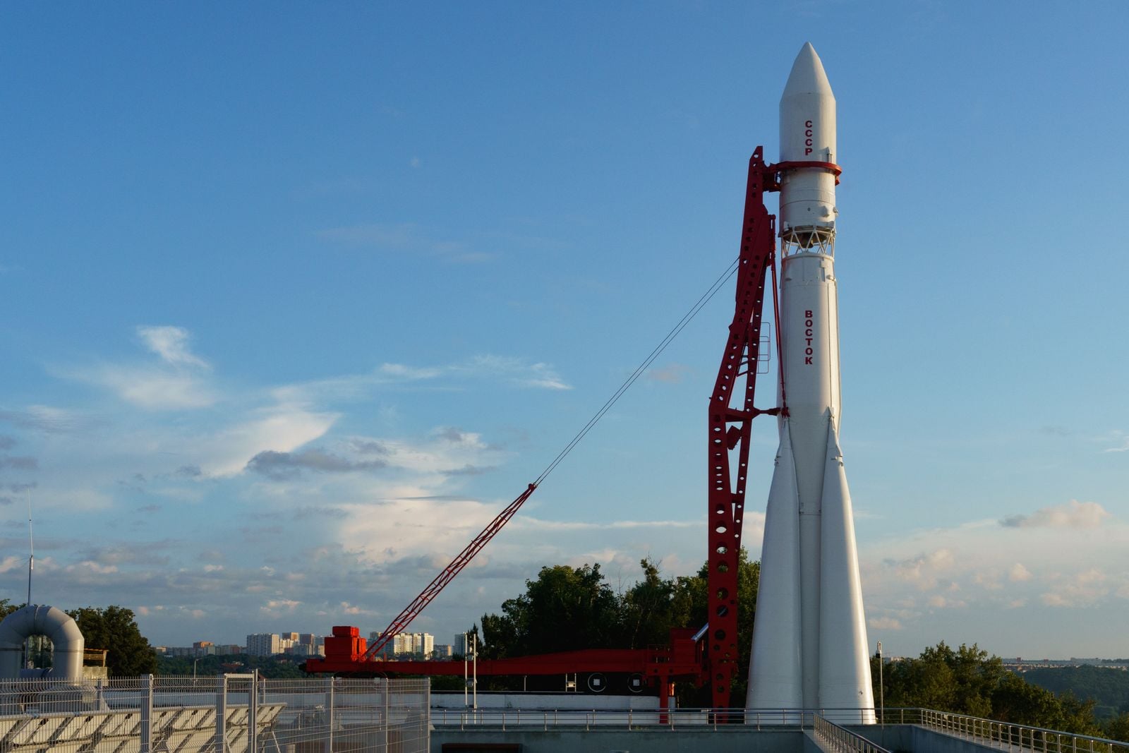
  •  

Psychology says the person in the friend group who never seems to need anything isn’t low-maintenance, they learned in childhood that having needs was the fastest way to become inconvenient

Psychology says the person in the friend group who never seems to need anything isn't low-maintenance, they learned in childhood that having needs was the fastest way to become inconvenient

Walk into any kitchen where a group of old friends has gathered, and you can spot them within ten minutes. The kettle is going, someone is loudly relitigating a bad date, someone else is asking whether the wine in the fridge is open. And then there is the quiet one at the end of the counter, refilling everyone else’s glass, remembering who takes oat milk, laughing at the right moments, needing absolutely nothing. They are the easiest person in the room. They are also, often, the most misunderstood.

The group has a name for this person. Low-maintenance. Chill. The reliable one. Sometimes it is said with affection and sometimes with a kind of relief, as though the rest of the group is grateful not to have to worry about them. What almost no one says out loud is that the person in question rarely worries about themselves in front of others either. They have made a lifelong practice of being the one who does not need much. And that practice, in most cases, started long before adulthood.

The friend who never asks for anything is usually the friend who learned not to

Psychologists who study attachment have a specific term for the pattern behind this. It is called avoidant attachment in childhood, and it often shows up in adulthood as a dismissive-avoidant style. According to clinical research summarised by psychologist Lisa Firestone, roughly 30 percent of people carry some version of this pattern, and it tends to develop when a child does not consistently feel safe, seen, or soothed by the adults raising them.

The child adapts by becoming what Firestone calls pseudo-independent. They meet their own needs, because depending on someone who keeps failing to respond is more painful than going without. Over time, they stop registering the needs at all. It is easier to feel nothing than to feel repeatedly disappointed.

By adulthood, this looks like competence. The person is efficient, self-contained, warm in a slightly reserved way. They rarely ask for favours. They rarely complain. When something is wrong, they process it privately and present the group with the finished thought. Everyone assumes this is temperament. Often it is training.

What actually happens in the child’s nervous system

The clearest picture of this pattern comes from a study designed in the 1970s by Mary Ainsworth, and it still holds up. In her Strange Situation experiment, a child plays with a parent in a room, the parent leaves, and the child’s response to the reunion is observed. A securely attached child gets upset when the parent leaves and seeks comfort when they return. An avoidant child appears unbothered when the parent leaves and does not seek comfort when they come back.

The catch is what the heart monitor shows. The avoidant child shows physiological signs of distress the entire time the parent is gone. The distress is there. It has simply been separated from any outward request for help. As contemporary attachment research puts it, the internal working model formed in these early years quietly guides expectations of self and others for decades afterward.

Translate that into a friend group in your thirties or forties. The person who never seems to need anything is not calm. They are regulated at the surface and activated underneath. The performance of being fine is so old and so practiced that even they cannot always tell the difference anymore.

The specific belief that keeps the pattern running

What the child learned was not simply that adults are unreliable. The child learned something more corrosive, which is that having needs made the adult withdraw further. So the needs themselves became the problem. Firestone describes the internal script bluntly: the child begins to believe they are not worth paying attention to, and disconnects from their wants to avoid the shame of them going unmet.

That belief does not evaporate at eighteen. It shows up at brunch, at group chats, at the office. It shows up as the friend who insists they are fine while going through a divorce. It shows up as the colleague who quietly absorbs an unreasonable workload and only mentions burnout after they have already accepted a job somewhere else.

The core conviction is not that other people are cruel. It is that having a need, out loud, is the fastest way to become inconvenient. And no one wants to be the inconvenient one.

Why this looks like a virtue from the outside

Culture rewards the low-maintenance friend. They get invited more, complained about less, and praised for being easy. In a world where many people are quietly carrying some form of insecurity, the person who asks for nothing feels like a gift.

But the reward system is part of the trap. Every time the friend group praises the quiet one for being so easy, it confirms the original lesson: your value here is your lack of need. This is how the pattern survives into middle age. It is being reinforced by the very relationships that are supposed to make the person feel safe.

It is worth saying plainly. Being easygoing is not the same as being avoidantly attached. Plenty of secure people are also low-drama. The difference is whether the person could ask for something if they needed to, and whether they would trust the room to respond. The avoidant friend usually cannot, and does not.

How it shows up in romantic relationships

The friend-group version is the softer face of the pattern. The romantic version is where it tends to break things. A February 2025 piece in Forbes on attachment and partner selection notes that people with a dismissive style tend to hold positive views of themselves and negative views of others, which reads at first like confidence but functions like a wall.

In a relationship, this looks like the partner who is present but somehow unreachable. They plan the holidays. They remember birthdays. They are physically there. And yet a partner can spend years feeling as though there is a room in the house they have never been allowed into. When the more expressive partner asks for closeness, the dismissive partner reads the request as neediness, dramatics, too much.

What makes it hard to name is that the dismissive partner is not consciously withholding. They are running the same program they ran at four years old, which is: notice nothing, need nothing, do not give the other person a reason to pull away. The tragedy is that this is often exactly what causes the other person to pull away.

The physical cost of never being inconvenient

Suppressing a need is not free. The nervous system still registers the want, still fires the stress response, still processes the disappointment. It just does so silently. Over time, this shows up as vague physical symptoms, sleep problems, low-grade resentment that has nowhere to go, and a strange sense of loneliness in rooms full of people who love you.

The loneliest people in midlife are often not the ones without partners or children. They are the ones surrounded by people who only know the version of them that shows up when everyone else needs something. The low-maintenance friend is often that person. Beloved, and unknown.

Why the pattern can pass to the next generation

Attachment researchers have found that the way a parent processes their own history matters more than what happened to them. If we do not make sense of and feel the full pain of our past, we are much more likely to repeat it. The parent who was raised in an emotional desert and never grieved that fact tends to raise a child in a slightly greener version of the same one.

The findings extend into how people build families in the first place. A study covered by Scientific American found that attachment style may even influence how many children people end up having, with insecure patterns correlating with different family sizes than secure ones. The influence runs deeper than most people realise.

This is not a life sentence. It is a pattern that responds to attention. But it does not respond to willpower or to being told to open up more. It responds to a slow rebuilding of the belief that a need, expressed out loud, will not cost the person the relationship.

What a secure version of this friend actually looks like

Descriptions of what secure attachment looks like in children tend to emphasise a specific balance. The child explores confidently and comes back for comfort when they need it. They do not have to choose between independence and closeness. They get both.

In adulthood, the secure version of the low-maintenance friend is still calm, still competent, still not prone to drama. But when something is genuinely hard, they say so. They do not perform crisis, and they do not perform fineness either. They tell one or two people what is going on, they let those people help, and they trust that the friendship will not shrink because of it.

The difference is small on the outside and enormous on the inside. One version is regulating alone in a room full of people. The other version is actually with them.

Signs the pattern is running, in a friend or in yourself

A few markers show up consistently. The person can list what everyone else in the group is going through, but goes vague when asked about their own life. They deflect care by redirecting the conversation. They apologise for taking up time before saying anything hard. When someone offers help, they refuse it reflexively, then feel a private flash of resentment that no one pushed harder.

Descriptions of the dismissive-avoidant style in adult partnerships often note this reflex specifically. The person genuinely believes they are protecting others by not burdening them, while the others often feel shut out by exactly this protection.

A more painful version of the same wiring, sometimes called fearful-avoidant attachment, involves wanting closeness intensely and pulling away from it in the same breath. The internal experience is exhausting. The external presentation, again, often looks like someone who simply does not need much.

How the pattern actually loosens

The change does not come from a dramatic disclosure. It comes from small experiments in being slightly more inconvenient than usual, and noticing that the room does not empty out. Saying, out loud, that you had a hard week. Asking a friend to come with you to an appointment. Letting someone drive you home when you could have taken a cab. These sound trivial. For someone whose nervous system was trained to hide need, they are not.

Firestone’s clinical work emphasises building what she calls a coherent narrative, which is essentially the ability to tell the story of what happened to you as a child without collapsing into it or dismissing it. People who can do this tend to raise more securely attached children, and tend to form warmer adult relationships, regardless of what they started with.

The friend group rarely notices the shift at first. What they eventually notice is that the quiet one at the end of the counter is talking a little more about themselves, asking for the thing they actually want, letting someone else refill their glass for a change. It looks like a personality change. It is closer to a homecoming.

A last thought about the person who never seems to need anything

If someone in your life fits this description, the useful move is not to interrogate them or to praise them harder for being so easy. It is to ask specific questions and to stay in the room when the answer is slow. What was hard about this week. What would actually help. What would you want if you thought you were allowed to want it. Then wait.

The person who learned early that having needs made them inconvenient did not choose that lesson. They inherited it from a room that could not hold them. A different room, decades later, can teach a different lesson. It just has to be willing to keep asking, and to mean it.

The post Psychology says the person in the friend group who never seems to need anything isn’t low-maintenance, they learned in childhood that having needs was the fastest way to become inconvenient appeared first on Space Daily.
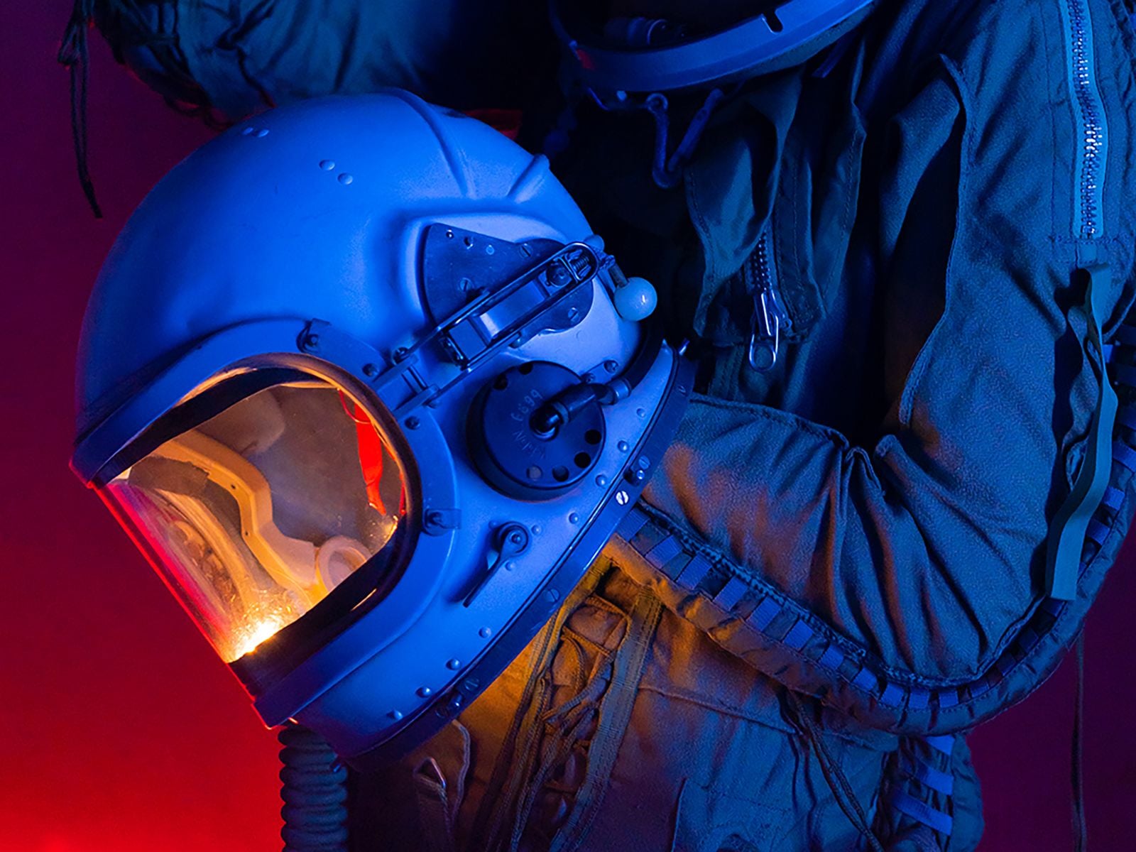
  •  

In September 1983, a Soviet lieutenant colonel named Stanislav Petrov sat in a bunker south of Moscow watching his early-warning screens light up with five incoming American missiles, and instead of phoning it up the chain he decided the computer was lying and waited — a judgment call that historians now credit with preventing a retaliatory nuclear launch

In September 1983, a Soviet lieutenant colonel named Stanislav Petrov sat in a bunker south of Moscow watching his early-warning screens light up with five incoming American missiles, and instead of phoning it up the chain he decided the computer was lying and waited — a judgment call that historians now credit with preventing a retaliatory nuclear launch

Just after midnight on 26 September 1983, an alarm sounded inside the Serpukhov-15 command bunker south of Moscow. A satellite feed from the Soviet Union’s new early-warning system, Oko, reported that the United States had launched a nuclear missile. Within minutes it reported four more. The officer on duty, Lieutenant Colonel Stanislav Petrov, had a screen in front of him with the word LAUNCH in Cyrillic, a bank of phones connecting him to the Soviet high command, and roughly the length of a coffee break to decide whether the warning was real.

He decided it wasn’t. He picked up the intercom to the operations duty officer and reported a system malfunction.

He was guessing.

Soviet bunker command console

What the screen actually said

The Oko constellation was Moscow’s answer to the American Defense Support Program satellites: a ring of spacecraft in highly elliptical orbits designed to spot the infrared bloom of a US intercontinental ballistic missile the moment its engines lit. The system had gone operational only months earlier. According to a HistoryExtra account of the incident, Petrov knew Oko was new and relatively untested, and that fact was doing quiet work in the back of his mind as the alarm escalated.

Protocol was unambiguous. A confirmed launch detection went up the chain immediately. From there, the Soviet doctrine of the day — launch on warning — would have compressed the decision window to minutes. The general staff would consult, wake Yuri Andropov if he wasn’t already awake, and either sit on the report or authorise a retaliatory salvo of hundreds of warheads at American cities and silos.

Petrov’s job was not to make that decision. His job was to pass the alert along cleanly, quickly, and without editorial. He did not do his job.

Why he thought the computer was lying

Two things nagged at him. The first was arithmetic. A genuine American first strike, in the Soviet threat models of 1983, would look like a wall — hundreds of missiles arriving in a coordinated wave designed to destroy Soviet retaliation capability before it could launch. Five missiles was not a decapitation strike. Five missiles was almost a taunt. As The Guardian noted in its obituary, Petrov reasoned that the shape of the attack made no strategic sense.

The second was the ground picture. Soviet over-the-horizon radars could not see American missiles until they crested the earth’s curvature, and at that moment those radars were showing nothing. Waiting for confirmation from ground radar meant burning the warning window down to almost zero. If the satellites were right and he waited, the Soviet Union would have only minutes to respond, and possibly not even that.

He waited anyway.

The room, the phones, the interval

The Serpukhov-15 bunker was not a small room with one man at a desk. It was a full command post, staffed with duty officers and analysts, and Petrov later described the atmosphere in the minutes after the first alert as loud and physically disorienting. The alarm was audible. Screens flashed. Junior officers around him were shouting numbers.

He held the intercom. He listened to the ground-radar operators reporting nothing. He counted the missiles as Oko reported them: one, then four more.

According to NPR’s account of the night, Petrov later said he had a funny feeling in his gut. That was the phrase he used. It is not the phrase military historians prefer. It is, however, the phrase that survived.

He reported a system malfunction to the operations duty officer. The report he filed said false alarm.

early warning satellite

What had actually happened

Investigators reconstructed the fault over the following weeks. The Oko satellites had been positioned to look at the horizon rather than straight down at American silo fields, a design choice that reduced background noise from Earth’s own thermal emissions. But it made the system vulnerable to a specific optical trick: sunlight at a shallow angle, reflecting off high-altitude clouds above North Dakota, hit the satellite’s infrared sensor with the same signature as a rocket exhaust.

Five reflections, five “missiles.” A weather artifact, dressed up by a young algorithm as the end of the world.

The engineers who built Oko later patched the system to cross-check any launch detection against geostationary satellite data before triggering the top-level alert. That patch existed because of the night Petrov spent staring at the screen.

How close it actually came

Historians and former Soviet officers have argued for decades about how close the world really came to launch. Petrov did not have his finger on any button. He was one node in a decision chain that included the general staff, the defence minister, and ultimately Andropov himself, and each of those nodes could in principle have declined to authorise a strike even if Petrov had passed the warning up.

But context mattered. Three weeks earlier, a Soviet Su-15 interceptor had shot down Korean Air Lines Flight 007 over Sakhalin, killing 269 people including a US congressman. Washington’s rhetoric had turned incandescent. Andropov, ill and paranoid, had spent the previous year convinced the Reagan administration was planning a genuine first strike, and had ordered the KGB to hunt for evidence of it under a programme codenamed RYaN. The Soviet posture in September 1983 was hair-trigger by design.

A warning delivered up that chain, into that room, on that night, would not have been filed and forgotten. Whether it would have produced a launch order is unknowable. That it might have is why the story persists.

What happened to Petrov afterwards

He was not decorated. He was interrogated. His superiors were embarrassed — the malfunction pointed at design failures in a system the Soviet military had just spent enormous sums fielding, and honouring the officer who exposed it would have been an implicit indictment of the engineers and generals who signed off on it. Yuri Votintsev, then commander of Soviet missile-defence forces, privately praised Petrov’s judgment and mentioned an award. The award never came.

Petrov was reprimanded on paperwork grounds: his log entries from the night were incomplete. He was reassigned to a less sensitive post and took early retirement in 1984, in part because the stress of the incident had contributed to a nervous breakdown. He lived out the rest of his life in a small apartment in Fryazino, a satellite town outside Moscow, on a modest pension, growing potatoes.

The incident stayed classified until the late 1990s, when Votintsev published a memoir mentioning it. Western journalists tracked Petrov down. He gave interviews reluctantly. He never claimed to have saved the world, and got irritated when interviewers tried to write him as a hero. He said he was doing his job — that his job included judgment, and that judgment had told him the computer was wrong.

He died in May 2017, aged 77, of pneumonia. A German friend, Karl Schumacher, found out months later, when he called that September to wish Petrov a happy birthday and was told by Petrov’s son that his father had already died. According to later reporting on the incident, the delay in the news reaching the wider world was itself a kind of coda: the man who may have prevented the end of civilisation had died without anyone outside his family noticing.

Why the story keeps getting retold

Space Daily has looked before at what Petrov’s night reveals about human judgment against automated systems, and at a similar moment aboard a Soviet submarine during the Cuban Missile Crisis, when Vasili Arkhipov refused to authorise a nuclear torpedo launch against American destroyers. Both stories share a shape: a single officer, a broken or misleading input, a rule that says escalate, and a person who declines.

The engineering point buried in the Petrov story is worth pulling out. Oko was not a bad system in principle. It did what it was designed to do — detect the infrared plume of a rising ballistic missile — and it did so within its physical envelope. The failure was in the confidence with which its output was treated. The Soviet doctrine of launch on warning assumed the satellites would only ever be wrong in one direction, missing real attacks. It did not adequately model what would happen when the satellites reported an attack that wasn’t there.

Every early-warning architecture built since has had to reckon with the same asymmetry. The American BMEWS radars in Greenland famously mistook the rising moon for a Soviet ICBM salvo in October 1960, and the fix there was similar in spirit to what Oko needed: cross-checking, corroboration, redundancy across sensor types. The North American Aerospace Defense Command has publicly discussed multiple false alerts in the 1970s and 1980s that were caught before they reached the level of a launch order.

The number to remember

Five. The system reported five American missiles. Not one, which might have been dismissed as a rogue launch or a test gone wrong. Not four hundred, which would have matched the Soviet mental model of a genuine first strike and would probably have been believed. Five — a number small enough to be plausibly a glitch, large enough to be plausibly a warning shot, and squarely inside the gap where a human being had to decide which.

Petrov decided glitch. He was right. If Oko had reported a single missile, or a hundred, the story ends differently — either dismissed at a lower level, or believed at a higher one. It was the specific number, and the specific man watching the specific screen at 00:15 Moscow time, that made the incident hinge.

He kept the intercom in his hand. He did not press it up the chain. The clouds over North Dakota drifted east. The sun climbed. The satellites recalibrated. The morning shift arrived at Serpukhov-15 to find their new early-warning system had, overnight, tried to end the world, and a middle-aged engineer with a headache had told it no.

The post In September 1983, a Soviet lieutenant colonel named Stanislav Petrov sat in a bunker south of Moscow watching his early-warning screens light up with five incoming American missiles, and instead of phoning it up the chain he decided the computer was lying and waited — a judgment call that historians now credit with preventing a retaliatory nuclear launch appeared first on Space Daily.

  •  

In 1966, the Soviet chief designer behind Sputnik, Gagarin’s flight, and the entire early space program died during routine surgery, and only then did the world learn his name was Sergei Korolev — for a decade Moscow had referred to him in print only as the Chief Designer, because the KGB feared the CIA would have him killed

In 1966, the Soviet chief designer behind Sputnik, Gagarin's flight, and the entire early space program died during routine surgery, and only then did the world learn his name was Sergei Korolev — for a decade Moscow had referred to him in print only as the Chief Designer, because the KGB feared the CIA would have him killed

On 14 January 1966, a 59-year-old man died on an operating table at a Moscow hospital during what had been scheduled as a routine procedure to remove a bleeding polyp from his intestine. Two days later, the Soviet newspaper Pravda ran an obituary with a photograph, and hundreds of millions of readers learned, for the first time, the name of the man who had built Sputnik, launched Yuri Gagarin, and beaten the United States to almost every early milestone of the space age.

His name was Sergei Pavlovich Korolev. Until that obituary, Soviet newspapers had only ever called him Glavny Konstruktor — the Chief Designer.

For roughly a decade, one of the most consequential engineers of the twentieth century had been, by state policy, an anonymous title. Gagarin knew him. Khrushchev knew him. The workers at the Baikonur Cosmodrome knew him. The Central Intelligence Agency did not.

The secrecy, and why Moscow kept it

The practice was not a rumour or a later embellishment. Fordham University historian Asif Siddiqi, whose NASA-published Challenge to Apollo: The Soviet Union and the Space Race, 1945–1974 remains the standard English-language account of the program, has said that a Soviet newspaper reader in the early 1960s would have encountered only Korolev’s title, never his name. The show Star City, a recent Apple TV series, dramatises the practice literally: a character is referred to throughout as the Chief Designer, and the production notes confirm the naming was drawn from the historical record rather than invented for effect.

The scale of the anonymity is easier to grasp by inversion. Wernher von Braun, Korolev’s American counterpart at Marshall Space Flight Center, appeared on the cover of Time and gave televised interviews explaining the Saturn rocket family. Von Braun’s face and voice were part of the American story. Korolev’s were state secrets.

When Gagarin flew on 12 April 1961, the world saw the cosmonaut. It did not see the man who had designed the R-7 rocket carrying him, chosen the launch window, and stood in the bunker at Baikonur listening to the countdown.

The official reasoning, as Soviet-era veterans of the program have described it since, was straightforward: a named Chief Designer was a targetable Chief Designer. The Soviets wanted him anonymous, on the view that if he became known, both his life and the space program would be at risk.

Whether the CIA would in fact have moved against Korolev is a claim that historians treat cautiously. What is documented is that Soviet security services behaved as if that risk were real, and that the anonymity was maintained with unusual discipline across state media, scientific publications, and Nobel Prize correspondence. The Nobel Committee reportedly asked, more than once, for the name of the person responsible for Sputnik so a prize could be awarded. Khrushchev is said to have replied that the achievement belonged to the entire Soviet people. No name was given. No prize followed.

The National Review obituary essay marking the fiftieth anniversary of his death notes that the same secrecy that shielded Korolev also denied him the international recognition his American rival received in life. Von Braun died in 1977 as a public figure. Korolev died in 1966 as a title.

Sergei Korolev portrait

Who Korolev actually was

He was born in 1907 in Zhytomyr, in what is now Ukraine — a fact that has become politically charged in recent years, with the Russian Foreign Ministry publicly disputing Ukrainian claims on his legacy as recently as 2023. He trained as an aeronautical engineer in Moscow and Kyiv, worked on early liquid-fuel rocket research in the 1930s, and in 1938 was arrested during Stalin’s Great Purge on fabricated charges of sabotage.

He was sent first to a gold-mining camp in Kolyma, one of the harshest sites in the Gulag system, where he lost most of his teeth to scurvy and nearly died. He was later transferred to a sharashka — a prison design bureau where technically skilled prisoners worked on military aviation projects under guard. He was not formally rehabilitated until 1957, the same year Sputnik went up.

The man who launched the space age had, twenty years earlier, been beaten by NKVD interrogators and left to freeze in a labour camp. Sputnik’s insistence on a 1-watt transmitter loud enough for ham operators worldwide to hear was Korolev’s doing — he wanted ordinary people, not just governments, to know the object was up there.

The R-7, Sputnik, and the run of firsts

The rocket that made all of it possible was the R-7 Semyorka, originally designed as an intercontinental ballistic missile capable of carrying a thermonuclear warhead to the continental United States. On 4 October 1957 a modified R-7 placed Sputnik 1 into orbit. On 3 November 1957 it lofted Laika. On 12 April 1961 it carried Gagarin. The same fundamental design, in updated form, still launches Soyuz crews to the International Space Station today — the longest-serving orbital launch vehicle family in history.

Between 1957 and 1966, Korolev’s bureau delivered the first artificial satellite, the first animal in orbit, the first human in orbit, the first woman in orbit (Valentina Tereshkova, 1963), the first multi-crew spacecraft (Voskhod 1, 1964), and the first spacewalk (Alexei Leonov, March 1965). A BBC Sky at Night Magazine profile of Korolev notes that this run of firsts was compressed into less than a decade, driven by a single bureau operating under a single technical director whose name the public was not permitted to know.

Gagarin, according to accounts published after Korolev’s death, referred to him in private simply as SP — the initials of his first name and patronymic. Even the cosmonauts used the euphemism.

The surgery that killed him

By late 1965, Korolev was 58, exhausted, and unwell. He had been complaining of intestinal bleeding. On 14 January 1966 he was admitted to a Moscow hospital for what was described as a routine polyp removal. The operation was performed by Boris Petrovsky, the Soviet Minister of Health. Once the surgery began, the situation worsened rapidly: the polyp turned out to be a large malignant tumour, and Korolev’s jaw — broken during his 1938 NKVD interrogation and never properly reset — could not be opened wide enough to intubate him for extended anaesthesia. He died on the operating table of heart failure.

He was 59. The Pravda obituary two days later carried his photograph and, for the first time in print, his full name and title. He was buried in the Kremlin Wall Necropolis. The state that had hidden him spent the following week publishing everything he had built.

Kremlin Wall Necropolis

What his death cost the program — and the record

The lunar program he had been directing — the N1 super-heavy rocket, the Soviet answer to the Saturn V — collapsed in the years after his death. All four N1 launches between February 1969 and November 1972 failed, most spectacularly the second attempt in July 1969, which destroyed the launch pad. The rocket clustered 30 NK-15 engines in its first stage because Korolev’s rival Valentin Glushko had refused to build larger engines using the propellants Korolev preferred; the KORD fault-management system meant to coordinate those 30 engines was defeated by electromagnetic interference between them, turning single-engine failures into cascade shutdowns.

Siddiqi, the Fordham historian, has offered the measured verdict that Korolev’s death had a very negative effect on the Soviet space program as a whole, including the lunar program, but that he doubted the Soviets would have made the Moon landing even if Korolev had lived, because so many structural and organisational problems were already present while he was alive.

That caveat is the one the alternate-history television now rests on. Star City, which premiered on Apple TV in 2026, is set in a timeline where the 1966 surgery does not kill him and Alexei Leonov walks on the Moon in 1969. The show’s dramatic engine is not that Korolev was a genius who could solve any problem, but that his survival was the necessary condition under which the program’s institutional pathologies could have been addressed at all.

One consequence of a decade of anonymity is that the Western intelligence picture of the Soviet space program was, for years, a picture without a face. CIA assessments through the late 1950s and early 1960s referred to the Chief Designer as a hypothesised figure whose existence could be inferred from the pattern of Soviet achievements but whose identity, nationality, and biography were unknown. Some analysts speculated the Chief Designer was a committee. Others suspected a captured German engineer. The correct answer — a Ukrainian-born, Gulag-surviving aeronautical engineer named Korolev — was not confirmed in the West until Pravda printed it.

Space Daily has written before about the Buran shuttle’s single 1988 flight, another Soviet program whose technical achievement was decoupled from public recognition by the state’s habits of secrecy. The pattern is older than Buran. It began with Korolev.

The anonymity also meant that when he died, the state had to invent his public identity retroactively. The Pravda obituary was the first time Soviet citizens saw the photograph of the man whose name had been on none of the achievements they had spent a decade celebrating. Schoolchildren who had memorised Gagarin’s flight learned, in one morning, that there had been a designer, that he had been Ukrainian-born, that he had been imprisoned by Stalin, and that he was already dead.

The name on the wall

Korolev’s ashes are interred in the Kremlin Wall, near Lenin’s mausoleum. A crater on the far side of the Moon carries his name. A city outside Moscow, formerly Kaliningrad, was renamed Korolyov in 1996. The Yuri Gagarin Cosmonaut Training Center at Star City — the real one, not the Apple TV version — still trains the cosmonauts who ride his rocket’s descendants to orbit.

The R-7 family, in its current Soyuz-2 configuration, has now flown more than 1,900 times across all variants since 1957. Every crewed launch from Baikonur since Gagarin has used a rocket that traces its lineage directly to the machine Korolev built to carry a hydrogen bomb.

The man’s name appeared in a Soviet newspaper for the first time on 16 January 1966. Sixty years later, it is on a Moon crater, a Russian city, and the side of every Soyuz that leaves the pad.

The post In 1966, the Soviet chief designer behind Sputnik, Gagarin’s flight, and the entire early space program died during routine surgery, and only then did the world learn his name was Sergei Korolev — for a decade Moscow had referred to him in print only as the Chief Designer, because the KGB feared the CIA would have him killed appeared first on Space Daily.

  •  

Mars is slowly pulling Phobos inward by about 1.8 centimetres a year; models suggest the battered moon could be torn apart in 20 to 40 million years, giving the planet a temporary ring

Representative rocky red landscape under a dark sky

Mars has no rings today, but it already carries the material for one.

Phobos, the larger and innermost of the planet’s two small moons, is moving towards Mars by about 1.8 centimetres each year. That drift is measurable. What happens at the end is modelled rather than observed, and depends heavily on how much strength is hidden beneath the moon’s battered surface.

One influential analysis suggests the weakest parts of Phobos could be pulled apart in 20 to 40 million years, spreading into a temporary ring while stronger fragments continue down towards Mars.

It is a dramatic future assembled from a very small motion.

Phobos completes three orbits during one Martian day

Phobos is an irregular body measuring roughly 27 by 22 by 18 kilometres. According to NASA’s Phobos overview, it circles Mars three times per day at an altitude of about 6,000 kilometres above the surface.

The European Space Agency gives its orbital period as 7 hours and 39 minutes. That is much shorter than the time Mars takes to rotate once. To an observer on much of the Martian surface, Phobos would therefore appear to rise in the west and set in the east, the reverse of the familiar daily motion of Earth’s Moon.

The short orbit is also the reason Phobos is in trouble. It lies inside the altitude where a moon’s orbital period would match the planet’s rotation. The tidal bulge it raises on Mars consequently lags behind the fast-moving moon. Their gravitational interaction removes orbital energy from Phobos and transfers it to Mars.

Losing orbital energy does not make a moon hover more slowly at the same height. It drops into a lower orbit, where it travels faster and raises stronger tides. The descent gradually accelerates.

A yearly drift cannot simply be extended in a straight line

NASA expresses the present decay as 1.8 metres every century, while ESA gives the equivalent figure of 1.8 centimetres per year. A simple division of the moon’s current altitude by that rate would produce a timescale of hundreds of millions of years.

That calculation is misleading because the rate will not remain constant. As Phobos approaches Mars, the strength of the tidal interaction increases. The last part of its inward spiral is expected to proceed much faster than the motion measured today.

This is why public estimates differ. NASA says Phobos could strike Mars or break into a ring in about 50 million years. ESA uses the broader phrase “within 100 million years.” These are not scheduled events with a precise date. They reflect different assumptions and levels of rounding applied to a nonlinear process over geological time.

The measured direction is the firm part: Phobos is moving inward.

The ring prediction depends on a damaged interior

Whether Phobos reaches the surface mostly intact or comes apart first depends on its internal strength. The moon has a nine-kilometre impact scar called Stickney crater, fine surface dust, grooves and evidence of repeated impacts. Its exterior looks less like a solid, pristine rock than an object that has been worked over for billions of years.

In a 2015 analysis published in Nature Geoscience, Benjamin Black and Tushar Mittal combined geological observations, spectral measurements, orbital theory and a geotechnical model of Phobos’s strength. They concluded that much of the moon may consist of weak, heavily damaged material.

Their model placed tidal dispersal of the weakest material about 20 to 40 million years in the future. Once Mars’s gravity pulls more strongly on the near side of Phobos than the moon’s own cohesion can resist, that material would no longer remain a single body.

This is one model, not a direct measurement of the interior. No spacecraft has drilled through Phobos or mapped its structure in full. A stronger, more coherent moon could survive closer to Mars, while a loose aggregate would begin failing farther out.

The grooves are intriguing, but they are not a visible countdown

Long grooves cross much of Phobos, and their origin has generated several explanations. Some have been linked to debris launched from impacts on Mars. Others may have been cut by boulders rolling away from Stickney crater.

A 2016 study in the Journal of Geophysical Research: Planets, led by Terry Hurford, tested another possibility. Its stress models found that tidal forces acting on a weak interior could produce fractures with a pattern similar to some observed grooves.

That does not establish that every groove is a stretch mark caused by orbital decay. Surface features can have several origins, and the competing explanations involve different sets of grooves. The study is better read as evidence that tidal damage is physically plausible for a weak Phobos, not that the moon is visibly splitting today.

At the present decay rate, human observations cover almost none of the remaining process.

A Martian ring could outlast species and still be temporary

Black and Mittal estimated that the resulting ring could persist for one million to 100 million years. Its initial mass density might be comparable with Saturn’s rings, although that does not tell us exactly how bright or broad it would appear from the Martian surface.

The ring would not be Phobos’s only ending. Material strong enough to avoid disruption would keep descending and eventually strike Mars in oblique, relatively low-speed impacts. Smaller particles in the ring would also evolve, collide and gradually move towards the planet.

On geological timescales, a ring lasting millions of years can still be a passing phase.

The contrast with Earth’s Moon helps show why. NASA’s lunar measurements show that our Moon is receding by about 3.8 centimetres per year. Earth rotates faster than the Moon orbits, so Earth’s tidal bulge transfers energy outward to the Moon. Phobos orbits faster than Mars rotates, reversing the exchange.

The same broad physics can push one moon away and pull another towards destruction.

Mars offers a ring system in slow preparation

Nothing about Phobos’s fate is urgent on a human scale. Twenty million years is more than four thousand times the span of recorded history. The moon will look effectively unchanged to any mission operating this century.

Its inward motion still matters because it lets planetary scientists observe one stage of a process otherwise inferred from finished ring systems, impact deposits and missing moons. Mars is not merely a planet that may acquire a ring in the distant future. It is a planet whose tides are already preparing the material.

The 1.8 centimetres measured in a year is almost nothing. Given enough time, it is the beginning of an ending.

The post Mars is slowly pulling Phobos inward by about 1.8 centimetres a year; models suggest the battered moon could be torn apart in 20 to 40 million years, giving the planet a temporary ring appeared first on Space Daily.
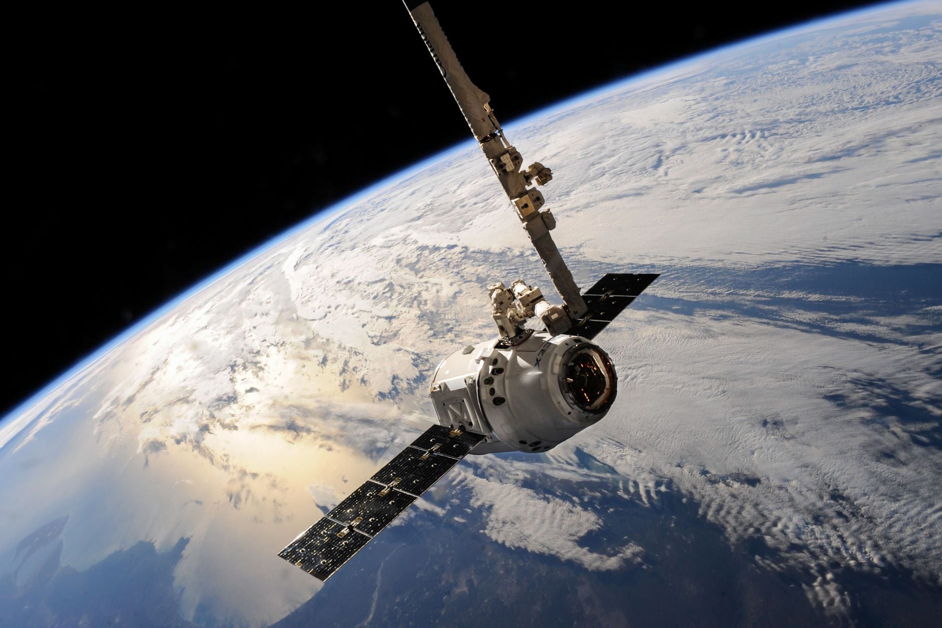
  •  

AI will not pilot future spacecraft like a human captain; its practical role is narrower and more important, choosing routes, spotting hazards and keeping missions working when Earth is minutes or hours away

Representative image of a satellite travelling above Earth

AI is likely to become important to future space travel for a fairly unglamorous reason: Earth is too far away to make every decision in time.

A spacecraft near Mars may wait minutes for a radio command. At the outer planets, the delay stretches into hours. A vehicle approaching an asteroid, descending towards unfamiliar ground or responding to a failing component may need to act before a human team can see the problem, discuss it and send an answer back.

That does not mean future spacecraft will be handed to a talking machine captain. On the evidence available today, the practical role is narrower: recognising a local situation, choosing among approved actions and keeping a mission working within limits set by people.

Spacecraft autonomy began before the current AI boom

NASA tested an onboard artificial-intelligence system on Deep Space 1 in 1999. The Remote Agent experiment received high-level goals, produced plans, executed them and responded to four simulated faults inserted by the mission team. It also encountered a software bug during its first run, a useful reminder that autonomy creates new failure modes as well as new capability.

Deep Space 1 separately tested autonomous optical navigation. The spacecraft photographed asteroids against background stars, calculated its position and commanded its ion propulsion without waiting for engineers to perform each navigation calculation on Earth.

These systems were not generative AI. They were purpose-built planning, diagnosis and navigation software, designed around a constrained mission. That distinction remains useful today.

I wrote earlier about how AI already flying in space tends to solve one specific physical problem. Future capability will probably grow by joining many such bounded systems, not by installing a single general intelligence and asking it to improvise.

DART showed why decisions sometimes have to stay onboard

NASA’s DART spacecraft had to strike Dimorphos, an asteroid moonlet roughly 150 metres across, while closing at about six kilometres per second. During the final phase, human intervention would have been too slow and the target did not separate clearly from the larger asteroid until late in the approach.

DART’s SMART Nav system used images from its camera to identify the bodies, select Dimorphos, calculate corrections and command manoeuvres. The system guided DART through the last four hours without human control, ending in the intended collision on 26 September 2022.

That is autonomy with a sharply defined objective.

The spacecraft was not deciding whether the mission was wise or inventing a new scientific goal. People had designed, tested and authorised the decision structure. The machine handled the part that had to occur faster than the radio link allowed.

Newer AI can assist with planning before it flies

In December 2025, NASA’s Perseverance team completed the first two drives on another world whose waypoints had been generated by AI. A vision-language model examined orbital imagery and elevation data, identified terrain features and proposed a route.

The AI was on Earth, not steering the rover live. JPL engineers ran its commands through a digital replica of Perseverance and checked more than 500,000 telemetry variables before transmission. The rover then drove 210 metres on 8 December and 246 metres on 10 December, according to JPL’s account of the demonstration.

This suggests a near-term division of labour. AI can examine large image sets, propose waypoints and reduce routine planning work. Engineers can test those proposals against mission rules. Onboard navigation can then handle nearby rocks and other hazards as the vehicle moves.

Each layer has a different job, and each can be checked differently.

Hera will test more autonomy around an asteroid

ESA’s Hera spacecraft is due to reach the Didymos system in November 2026 to examine the aftermath of DART’s impact. ESA describes Hera as having autonomy comparable to a self-driving car, although the comparison refers to sensor fusion and local navigation rather than road-driving software transplanted into space.

Hera will combine camera images, laser-altimeter readings, inertial sensors and star-tracker data to build a working picture of the two asteroids. Its experimental modes are intended to recognise surface features and make navigation decisions near bodies whose weak gravity and irregular shapes are difficult to model perfectly from Earth.

If those tests work, the same broad approach could help later spacecraft rendezvous with small objects, inspect damaged satellites or land in places where detailed maps are incomplete. It would be evidence for particular navigation methods, not proof that a spacecraft can manage an entire mission alone.

Future travellers will need systems that know their authority

For robotic probes, autonomy can mean more observations and less time waiting. For crews, it could help monitor equipment, flag anomalies, manage inventories or compare possible responses while Earth is unavailable. Yet a system making suggestions for astronauts is not the same as one controlling life support or propulsion, where an error could be irreversible.

The harder engineering question is therefore not simply how capable the AI becomes. It is how its authority is bounded, how uncertainty is displayed, what happens when sensors disagree and how people regain control.

I recently looked at the much larger physical barrier in the possibility of sending a probe to Alpha Centauri. AI cannot provide the propulsion, shielding or energy such a mission lacks. It could, however, help a small vehicle operate for decades without expecting Earth to supervise every choice.

That is the credible future role: not replacing mission control, but carrying a carefully tested part of mission control aboard the spacecraft when distance makes immediate help impossible.

The post AI will not pilot future spacecraft like a human captain; its practical role is narrower and more important, choosing routes, spotting hazards and keeping missions working when Earth is minutes or hours away appeared first on Space Daily.

  •  
❌