❌

Reading view

Extragalactic Planetary Nebula with Massive Progenitor Sheds Light on Stellar Evolution

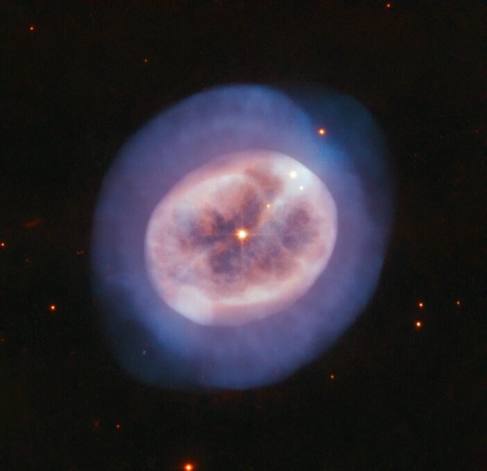
planetary nebula NGC 2022

Editor’s Note: This article was co-written by Lucas Brown and Alexia Kubas, our 2026–2027 AAS Media Fellows. We’re excited to welcome Lucas and Alexia to the team and look forward to featuring their writing on AAS Nova regularly!

Planetary nebulae mark a key evolutionary phase for low- and intermediate-mass stars, but properties of the parent star are difficult to sleuth out. Researchers have discovered an extragalactic planetary nebula in the center of a star cluster, offering an unprecedented opportunity to trace planetary nebula properties to parent star stats.

The Puzzle of Planetary Nebula Progenitors

A planetary nebula, so named because the first ones discovered resemble the planet Uranus in a small telescope, forms when a Sun-like star runs out of fuel and sheds its outer layers, leaving a hot remnant core enveloped in a gaseous nebula. At higher masses, a different process kicks in: stellar cores can collapse to produce a chaotic burst of stellar material called a supernova. Where exactly the boundary should be placed between planetary nebula progenitors and supernova-forming stars remains an outstanding question in the field of stellar evolution.

Answering this question is challenging because once a planetary nebula becomes visible, the progenitor star’s transition into a hot, compact white dwarf is already underway, making it difficult to determine the star’s initial mass. For this task, researchers seek out planetary nebulae within open clusters — groups of stars that were born from the same molecular cloud and are roughly the same age — so that cluster characteristics can help piece together the progenitor puzzle. Since open clusters tend to be relatively young, they are also a great tool to probe planetary nebulae from more massive progenitors and explore the boundary between stars that produce planetary nebulae and those that go supernova.

Striking Gold

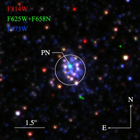
planetary nebula M279 in Andromeda

Open cluster AP 210 and planetary nebula M279 in the Andromeda Galaxy, as seen in archival Hubble observations. Click to enlarge. [Chen et al. 2026]

Numerous planetary nebula–open cluster pairs have been found in the Milky Way, but among those with well-constrained progenitor masses, very few push into the higher-mass regime where things get really interesting. Outside our home galaxy, the search has proven even more challenging due to data sparsity. Despite the odds, Pinjian Chen (Chinese Academy of Sciences) and collaborators have found a planetary nebula with one of the highest known progenitor masses in an open cluster in the Andromeda Galaxy.

To make this identification, Chen’s team used archival Hubble Space Telescope and MMT data to examine the location of the planetary nebula candidate M279 within the Andromeda Galaxy. The researchers’ critical observation was that the nebula not only overlaps with the position of an open star cluster called AP 210, but it also has an estimated velocity that matches the velocity of other stars in the cluster. These associations, when combined, provide strong evidence that M279 originated within the cluster.

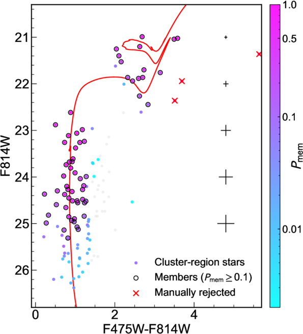
color–magnitude diagram for open cluster AP 210

Color–magnitude diagram of stars in the open cluster AP 210. Colored dots represent stars, and the red line is the best-fitting isochrone, which was used to determine the cluster’s age. Click to enlarge. [Chen et al. 2026]

What’s My (Cluster) Age Again?

M279’s cluster origin has significant consequences for pinning down the properties of the progenitor star. First, stars in open clusters all form at roughly the same time — 90 million years ago in the case of AP 210 — allowing the authors to set a tight constraint on the progenitor’s age. Then, because the rate at which a star burns through its nuclear fuel and generates a planetary nebula is related to its initial mass, the researchers are able to connect this age to a specific progenitor mass of around 5.7 solar masses.

The team also subtracted the central star’s contribution from the observed spectrum to isolate the nebula’s composition, illuminating specific nuclear processes relevant to higher-mass stars. Planetary nebulae are cosmic cocktails whose chemical abundances trace the composition of the interstellar medium when the progenitor formed as well as elements formed via nucleosynthesis inside the star during its lifetime. Chen and collaborators found the nebula to be significantly nitrogen-enhanced, which is consistent with a massive asymptotic giant branch progenitor undergoing hot bottom burning that converts carbon to nitrogen. This newly minted metal would then be mixed back into the star’s outer layers, flooding the resultant nebula with its particular spectral signature.

While this work represents only a single observation of a high-progenitor-mass planetary nebula — and only the third compelling extragalactic planetary nebula–open cluster pair — it opens up the possibility that there may be many more waiting to be found, unlocking new insight into the lives of massive stars.

Citation

“A Planetary Nebula from a 5.7 M⊙ Progenitor in a 90 Myr M31 Star Cluster,” Pinjian Chen et al 2026 ApJL 1005 L2. doi:10.3847/2041-8213/ae77e4

The post Extragalactic Planetary Nebula with Massive Progenitor Sheds Light on Stellar Evolution appeared first on AAS Nova.

  •  

Upper Limits on Planet-Induced Gigahertz Radio Emission from Inactive M Dwarfs

Jackie Villadsen et al 2026 ApJ 1005 51

No bursty radio emission characteristic of star–planet interaction was detected from a sample of five M dwarfs with close-in terrestrial planets, but researchers were able to place limits on the magnetic fields of the planets.

The post Upper Limits on Planet-Induced Gigahertz Radio Emission from Inactive M Dwarfs appeared first on AAS Nova.

  •  

Dust Deal with It

zodiacal light

Editor’s Note: Astrobites is a graduate-student-run organization that digests astrophysical literature for undergraduate students. As part of the partnership between the AAS and astrobites, we occasionally repost astrobites content here at AAS Nova. We hope you enjoy this post from astrobites; the original can be viewed at astrobites.org.

Title: The Exozodi Spectral Effect: Residual Habitable Zone Dust May Bias exoEarth Characterization
Authors: Miles H. Currie et al.
First Author’s Institution: NASA Goddard Space Flight Center
Status: Published in AJ

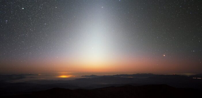
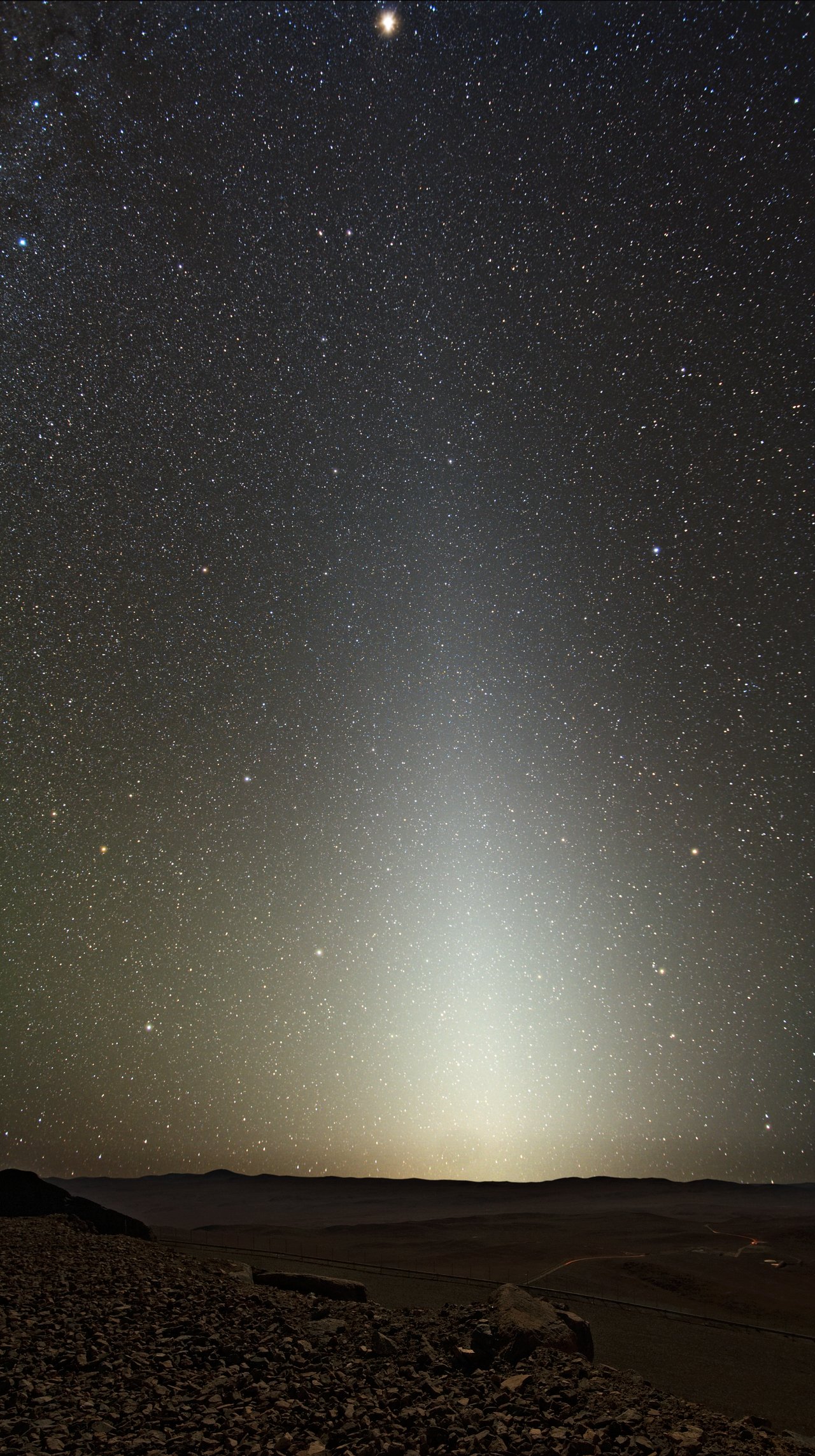
Figure 1: Zodiacal light as seen from Cerro Paranal. [ESO/Y. Beletsky; CC BY 4.0]

We have dust in our solar system — a huge cloud of it that permeates every corner. The dust itself is thought to be the product of many different processes including comet tails, collisions between asteroids, leftover debris from planetary formation, and gravitational collisions induced by planets. It’s small (on the order of 10–100 microns), made up of different silicates, and creates a noticeable triangle-shaped light that can be seen on the darkest nights (see Fig.1). This zodiacal dust is aptly named since the scattered light from the dust grains follows the line of the zodiac, or the ecliptic plane, across the sky. Its structure is quite complicated, with dust rings and trails and clumps near larger planetary bodies. For more information on the solar system’s zodiacal dust, you can read these bites here and here!

This zodiacal dust is not exclusive to the solar system. Other star systems, such as Tau Ceti and Vega, have been found to host similar clouds of interplanetary dust. This means planets imaged in these systems will also have emission from this dust mixed into the light that we observe from the planets. The Habitable Worlds Observatory (HWO) is a future space telescope mission under development by NASA. One of its primary science goals is to directly image 25 Earth-like planets in the habitable zones of nearby stars and look for signs of life (or biosignatures) in these planets’ atmospheres. Exozodiacal dust (aka exozodi) represents the biggest source of astrophysical noise that will need to be subtracted out from HWO observations of exoEarths. The authors of today’s article look at the potential impact of exozodi emission on the spectra of exoEarth atmospheres.

exozodiacal dust models

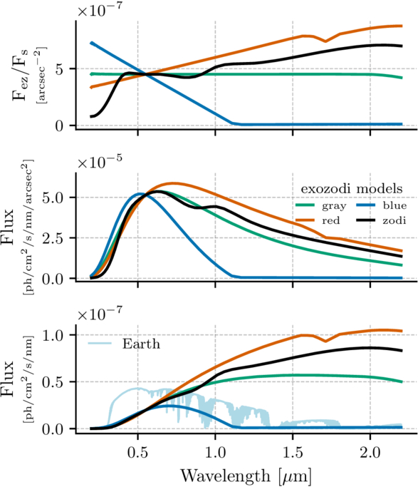
Figure 2: Different models of three “zodis” of dust observed at an inclination of 60 degrees plotted across HWO’s potential wavelength range. The gray scattering model is shown in green, the solar system’s model is shown in black, with the red and blue debris disk models shown in their respective colors. The top panel shows the flux contrast between the dust and the star. The middle panel shows the flux per area. The bottom panel shows the total flux captured with a 7.2-meter HWO with the thin blue line representing the spectrum of an Earth twin 10 parsecs (33 light-years) away for comparison. [Currie et al. 2026]

Show Me the Zodi

The authors first assume four different models of exozodi dust and how the dust’s emission changes with wavelength. The first model assumes a dust cloud that acts as a gray scatterer, meaning the particles scatter all wavelengths of light with no preference, and the second model’s dust acts just like the solar system’s does. However, it’s unknown whether the composition of exozodi will be the same as the solar system’s. Therefore, they adopt two more models of exozodi that act just like debris disks that have different compositions. One model is bluer in color because it is made up of smaller particles that preferentially scatter blue light, and the other model is redder in color because it is made up of bigger dust particles or different chemical compositions. Each of these models over HWO’s wavelength range can be seen in Figure 2. The authors then simulate a modern Earth atmosphere (both clear and 50% cloudy) as well as an Archean Earth atmosphere to understand how different exozodi models will affect observations of different exoplanet atmosphere conditions and compositions.

There’s Dust in My Spectra

In general, the effect that zodiacal dust has on the spectra of Earth-like planets can be broken down into two categories: its effect on the continuum and on the spectral features. The continuum is the object’s light emitted over all wavelengths and uninterrupted by spectral features. Spectral features are absorption and emission lines. These create either a dip or peak in the spectrum where atoms have either absorbed or emitted light at that particular wavelength. Lines at specific wavelengths tell us that a certain material is there, providing a list of possible chemicals that could be present in the planet’s atmosphere. For a brief summary of spectroscopy more generally, see here.

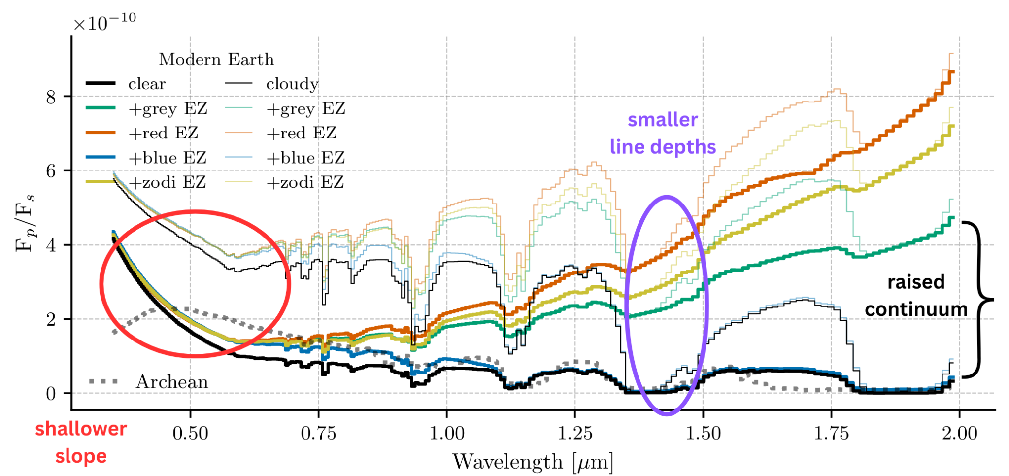
In the case of the continuum, exozodiacal emission raises the continuum, meaning the base flux of the planet is raised and absorption lines become more shallow. These effects can be seen in Figure 3, where the authors’ simulated spectra are plotted with and without zodiacal dust included. Not only is the continuum elevated for all models including zodiacal dust, notice how the dips become shallower at longer wavelengths. Because dust primarily radiates thermally, the red debris disk model nearly smooths out all dips beyond 1.25 microns! Molecules that absorb at these longer wavelengths, such as water or methane, may not be correctly identified with this type of exozodiacal emission.

simulated spectra of Earth-like planets with varying atmospheres and types of exozodiacal dust

Figure 3: Spectra of simulated modern-Earth atmospheres for clear (solid bright lines) and cloudy (solid dimmer lines) scenarios. The Archean Earth atmosphere is plotted in dotted gray. The redder exozodiacal spectrum has an elevated continuum and smoothed spectral features as opposed to the original, zodi-free spectrum plotted in black. [Currie et al. 2026, with annotations by Kaz Gary]

Additionally, the slope of the spectra between 0.25 and 0.75 microns (called the Rayleigh scattering slope) becomes shallower with zodiacal dust emission, which may bias our models toward lower-molecular-weight atmospheres. The slope at these wavelengths is dependent on the size distribution of molecules in the atmosphere, meaning it can tell us how much the average molecule in an atmosphere weighs.

From Figure 3, the effects of zodiacal dust are minimized with a bluer zodiacal dust model. This means systems with “bluer” zodiacal dust may be more optimal for HWO observations, as bluer dust does not scatter as much starlight as gray, solar system–like, or red dust. From their results, the authors recommend that the residual exozodi-to-planet flux ratio (in the V-band wavelengths) be kept to less than 10-2 in order to correctly understand the line depths (identify if a molecule is present or not) and 10-3 in order to accurately retrieve molecular abundances (understand how much of a molecule is present in the atmosphere). Dust is pesky enough here on Earth, but to find life on another planet like ours, we’ll dust have to deal with it.

Original astrobite edited by Anavi Uppal.

About the author, Kaz Gary:

I am a fourth-year PhD candidate at The Ohio State University with a passion for planets. My current work focuses on modeling exoplanet observations for the Habitable Worlds Observatory and understanding planetary atmospheres. Outside of research, I help develop planetarium shows and love all forms of science communication. In my free time, I enjoy playing tabletop RPGs, painting, watching terrible reality TV, and hanging out with my pet hedgehog.

The post Dust Deal with It appeared first on AAS Nova.

  •  

The Nineteenth Data Release of the Sloan Digital Sky Survey

SDSS Collaboration et al 2026 ApJS 285 9

For nearly three decades, the Sloan Digital Sky Survey has collected photometric and spectroscopic data for millions of objects; this article describes the most substantial data release to date for SDSS-V.

The post The Nineteenth Data Release of the Sloan Digital Sky Survey appeared first on AAS Nova.

  •  

Welcome and Farewell to Our AAS Media Fellows

logo of the American Astronomical Society

In 2017, we announced a new AAS-sponsored program for graduate students: the AAS Media Fellowship. This quarter-time opportunity is intended for current graduate students in the astronomical sciences who wish to cultivate their science-communication skills. This year, for the first time, we are welcoming two Media Fellows to the team.

We are pleased to announce that Lucas Brown and Alexia Kubas have been selected as our AAS Media Fellows for 2026–2027.

Alexia Kubas

Alexia Kubas, a 2026–2027 AAS Media Fellow, is a graduate student at Cornell University.

Alexia majored in astronomy with minors in physics, math, and planetary sciences at the University of Arizona. They are now a fifth-year PhD candidate at Cornell University, researching periglacial processes on Earth and Ceres. Outside of research, Alexia founded and currently helps run an Ithaca, NY, chapter of Astronomy on Tap.

Lucas majored in physics with an astronomy concentration at the University of California, Davis, and he has a master’s degree in physics from Tufts University. He is now a physics PhD candidate at the University of California, Santa Cruz, where he works with Stefano Profumo on studying the phenomenology of primordial black holes. Outside of research, Lucas participates in outreach activities through organizations like the Santa Cruz Organization for Outreach in Physics and the Project for Inmate Education. He also serves as co-chair of the Astrobites collaboration.

Lucas Brown

2026–2027 AAS Media Fellow Lucas Brown is a graduate student at the University of California, Santa Cruz.

As AAS Media Fellows, Alexia and Lucas will regularly write and publish summaries of the latest astronomy research on AAS Nova, assist in managing the distribution of press releases as part of the AAS press office, and gain a broad understanding of the worlds of scientific publishing, communications, and policy. Alexia and Lucas will also be assisting with the press conferences at the upcoming AAS meetings, so please say hello if you spot them at future meetings!

As we welcome our new Fellows to the team, we’ll also soon bid farewell to Lexi Gault, our 2024–2026 AAS Media Fellow. Lexi will be continuing her PhD research at Indiana University, where she studies the interstellar medium conditions in nearby low-mass galaxies. After defending her PhD in Spring 2027, Lexi plans to pursue a postdoc in extragalactic astronomy or a full-time science writing position.

Please join us in welcoming Lucas and Alexia as our new Media Fellows and wishing Lexi the best in all her future endeavors!

The post Welcome and Farewell to Our AAS Media Fellows appeared first on AAS Nova.

  •  

A Comparison of Lunar AI-Based Crater Databases Using Uniform Criteria

Stuart J. Robbins and Rachael H. Hoover 2026 Planet. Sci. J. 7 164

A uniform analysis of crater catalogs finds that practically all computer-generated catalogs return worse metrics than manually generated catalogs, though most catalogs do well in some areas and poorly in others.

The post A Comparison of Lunar AI-Based Crater Databases Using Uniform Criteria appeared first on AAS Nova.

  •  

Breaking the Ice: Origins of Carbon Oxides on Uranian Moons

Uranus close-up

For decades, astronomers have tried to decipher the source of carbon oxides on Uranus’s largest moons from ground-based telescopes. A recent study has leveraged JWST spectroscopy and laboratory experiments to identify carbon oxides and their origins for Ariel, Umbriel, Titania, and Oberon.

Unknown Origins of Carbon Oxide Enrichment

Forty years ago, the Voyager 2 spacecraft flew past Uranus and its twenty-seven moons, sending back prized portraits of the planet’s large and tidally locked satellites Miranda, Ariel, Umbriel, Titania, and Oberon. These images revealed extensive valleys, smooth plains, deep canyons, and possible icy volcanic (cryovolcanic) activity across the surfaces of the icy moons — the telltale signs of intense geologic activity. While Voyager 2 could take spectacular pictures, the spacecraft was not capable of identifying the molecules and materials making up these active surfaces.

Six largest moons of Uranus

Voyager 2 images of Uranus’s six largest moons. Click to enlarge. [NASA / JPL-Caltech / Ted Stryk; CC BY-NC-ND 4.0]

In the decades that followed, astronomers have used ground-based near-infrared spectroscopy of these moons to investigate their chemical compositions. These observations have detected weak carbon dioxide and hints of carbon monoxide ice features on the moons with clear spatial trends across the moons’ surfaces, but the origins of these carbon oxides remain unknown. There are two potential explanations for the presence of these molecules: 1) carbon oxides are native to the Uranus system, present from formation, or 2) they formed via radiolysis, in which charged particles trapped in Uranus’s magnetic field interact with water ice and carbon-bearing molecules on the moons’ surfaces.

Ground-based detections are limited due to contamination from Earth’s atmosphere as well as the overall weakness of the carbon dioxide spectral features, thus space-based near-infrared observations of the Uranian moons are necessary to better constrain the carbon oxides on the satellites. Luckily, JWST’s Near-Infrared Spectrograph (NIRSpec) now offers astronomers unimpeded access the moons’ carbon oxide spectral features.

Chemical Clues from Space and in the Lab

In 2024, a study acquired NIRSpec observations of Uranus’s moon Ariel, revealing prominent carbon dioxide features and confirming the presence of carbon monoxide ice hinted at by ground-based studies. Expanding on these observations to include Umbriel, Titania, and Oberon alongside Ariel, Richard J. Cartwright (Johns Hopkins University) and collaborators obtained JWST NIRSpec spectroscopy of Uranus’s four largest moons in hopes of disentangling the origin story of their carbon oxides.

Leading and trailing diagram

Diagram illustrating the leading and trailing sides of a moon orbiting Uranus. Click to enlarge. [AAS Nova/Kerry Hensley]

In addition to the JWST spectra, Cartwright and team performed laboratory experiments measuring the spectral properties of carbon dioxide ice over a range of very low temperatures (tens of kelvin). These experiments provided a better understanding of the spectral properties and nature of carbon dioxide on the surfaces of the Uranian moons. Comparing the JWST spectra with the laboratory spectra, the authors found that Ariel, Umbriel, Titania, and Oberon exhibit a variety of spectral features resulting from carbon dioxide ice, carbon monoxide ice, and other carbon-bearing molecules. The presence of these molecules varies between the leading and trailing hemispheres of the moons, these variations appearing strongest in Ariel and Umbriel. The carbon dioxide and carbon monoxide spectral features are stronger on the trailing hemispheres, decreasing with increasing distance from Uranus for all four moons.
spectral ratios

Spectral ratios of the trailing and leading hemispheres for each moon, labeling spectral features of multiple carbon-bearing molecules. Click to enlarge. [Cartwright et al 2026]

Carbon Oxide Origins

What does this mean for the origins of the carbon oxides on the Uranian moons? Spectral features of carbonate minerals and the widespread presence of carbon dioxide throughout the Uranus system suggest that these compounds exist natively. On the other hand, the concentration of carbon oxide features on the trailing hemispheres supports radiolytic production as these hemispheres are bombarded with more ionizing particles from Uranus’s magnetosphere.

Based on these results, the authors have postulated that both origin scenarios, native presence and radiolysis, are required to fully explain the presence of carbon oxides. Future laboratory studies and JWST observations will continue to reveal the nature and composition of bodies in the Uranus system, furthering our understanding of our solar system siblings.

Citation

“Tracing the Source of Carbon Oxides on the Large Moons of Uranus,” Richard J. Cartwright et al 2026 Planet. Sci. J. 7 199. doi:10.3847/PSJ/ae8818

The post Breaking the Ice: Origins of Carbon Oxides on Uranian Moons appeared first on AAS Nova.

  •  

Four-Body Gravitational Microlensing Events Involving Both a Binary Lens and a Binary Source

Cheongho Han et al 2026 ApJ 1004 183

Three newly characterized microlensing events augment the growing list of events involving binary sources and lenses, emphasizing the importance of testing models of this complexity.

The post Four-Body Gravitational Microlensing Events Involving Both a Binary Lens and a Binary Source appeared first on AAS Nova.

  •  

Discovery of Sulfur Oxides in the Ejecta of a B[e] Supergiant

Cristobal Bordiu et al 2026 ApJL 1005 L34

Researchers have detected SO and SO2 for the first time in an early-type evolved star; these results suggest that B[e]supergiants could be useful for studying sulfur chemistry under extreme radiation conditions.

The post Discovery of Sulfur Oxides in the Ejecta of a B[e] Supergiant appeared first on AAS Nova.

  •  

When Bright Spots Go Dark

solar faculae and sunspots imaged at 1400 Angstroms

Light and dark regions speckle the Sun and other stars, complicating the interpretation of exoplanet transmission spectra. New modeling suggests that faculae — bright areas on the visible surface of the Sun — appear dark on cooler stars, adding a new wrinkle to this challenge.

Dark Spot, Bright Spot

solar granules

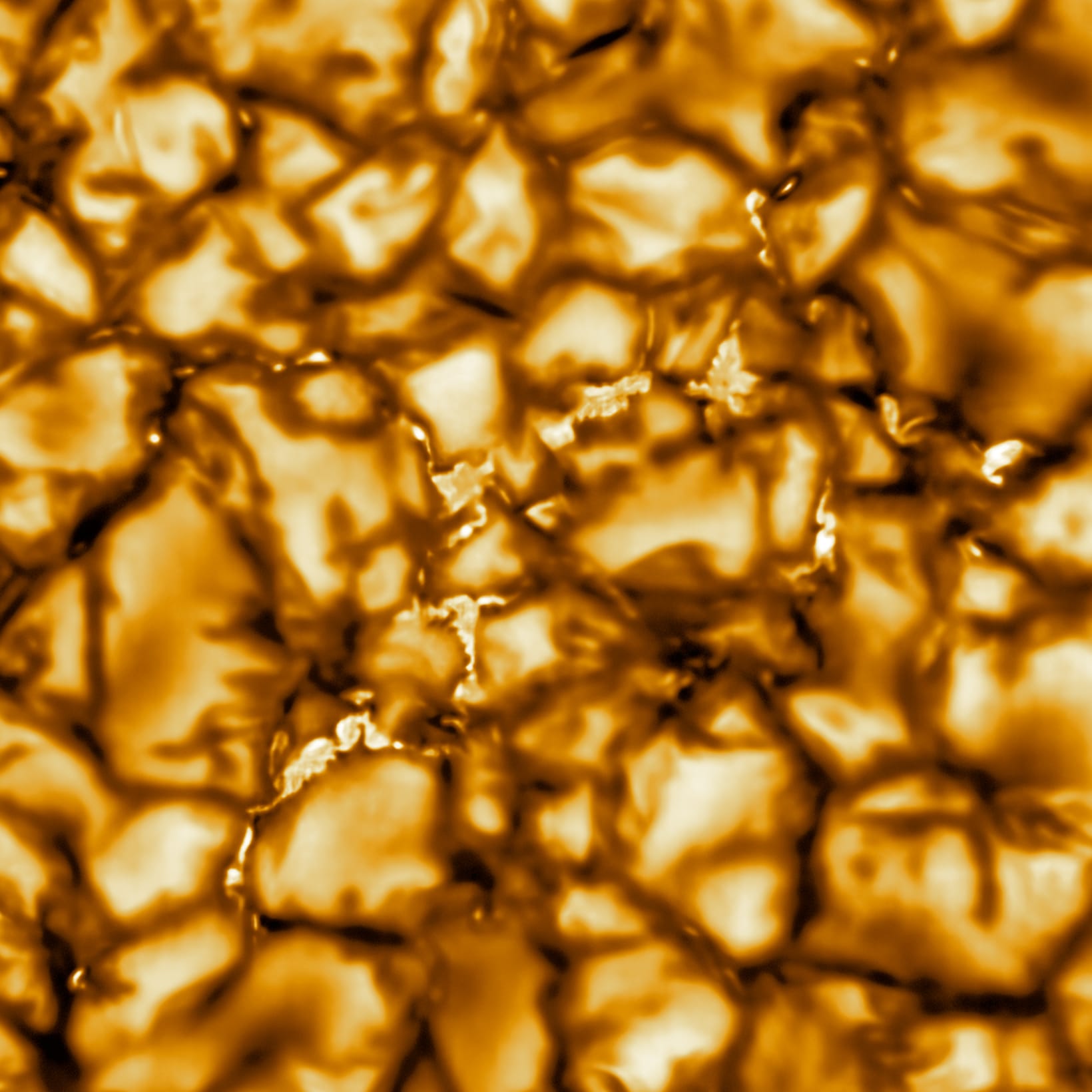
This image from the Daniel K. Inouye Solar Telescope shows solar convective cells called granules. The bright points in the dark lanes between granules are regions of enhanced magnetic field strength. [NSO/AURA/NSF; CC BY 4.0]

It’s an adage as old as exoplanet science itself: know thy star, know thy planet. This recommendation is key when using transmission spectroscopy to tease out the components of an exoplanet’s atmosphere; the backdrop to this process is a rotating star dotted with ever-changing active regions, and the better the star’s behavior is understood, the more reliable the extracted spectrum becomes.

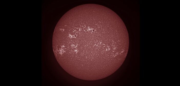
The Sun is freckled with dark spots — sunspots — as well as bright regions called faculae. Sunspots form where the Sun’s magnetic field bubbles up, creating pockets of cooler, less luminous plasma. Solar faculae form in regions of concentrated magnetic field, creating bright spots that line the dark crevasses between convective cells.

Other stars also have starspots and faculae, but thus far, astronomers have no direct observations of faculae on any star except the Sun. Out of necessity, researchers interpreting exoplanet spectra assume that faculae on other stars are similar to those on the Sun — but are they actually?

Would a Facula on Any Other Star Look as Bright?

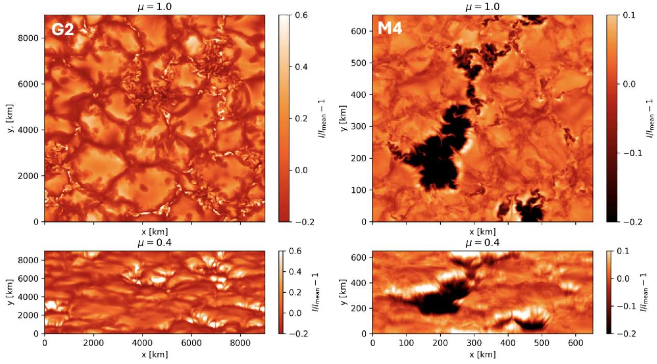
To explore what faculae might look like on stars other than the Sun, Alexander Shapiro (University of Graz; Max Planck Institute for Solar System Research) and collaborators turned to three-dimensional radiative magnetohydrodynamics simulations and radiative transfer modeling. Their aim was to simulate the appearance and spectra of faculae on stars of spectral type G2, K2, M0, and M4 — from Sun-like to substantially smaller and cooler than the Sun.

simulated faculae on a Sun-like star and a cooler M dwarf

Simulated faculae on a Sun-like star (left) and an M4 star (right). These images show the faculae at 600 nm. Click to enlarge. [Shapiro et al. 2026]

The modeled faculae on the Sun-like G2 star were bright, as expected. On the K2 and M0 star, these features were fainter, with the faculae on the M0 star being roughly as bright as the surrounding stellar surface. On the M4 star, the faculae were darker than surrounding areas, upending the assumption that faculae on all stars are brighter than the stellar surface.

Exoplanetary Effects

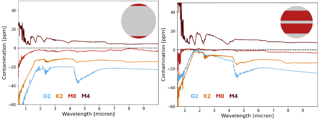
The transition from bright faculae on Sun-like stars to dark faculae on M4-class stars directly affects interpretations of exoplanet transmission spectra. The existence of dark faculae increases the derived exoplanet radius, whereas bright faculae on Sun-like stars decrease the derived radius. The contamination due to the faculae is wavelength dependent, with the largest contamination occurring at shorter wavelengths. This contamination, if not fully accounted for, can mimic spectral features from an exoplanet’s atmosphere.

plot of spectral contamination due to faculae

Contamination of transmission spectra by faculae near a star’s poles (left) and closer to the star’s equator (right). Faculae are bright for the simulated G2, K2, and M0 stars, and they are dark on the simulated M4 star. Click to enlarge. [Shapiro et al. 2026]

What determines whether faculae appear brighter or darker than their surroundings? Using a qualitative framework, Shapiro and coauthors found that the appearance of faculae can be traced to a few competing factors: the strong magnetic fields within faculae prevent the incursion of hotter material (making the spots appear darker), while the magnetic field lowers the opacity of the gas in that region, allowing us to peer deeper and glimpse hotter material (making the spots appear brighter). On cooler stars, effects related to higher surface gas pressure tilt the balance in favor of darker faculae.

Citation

“The Curious Case of Dark Faculae on M Dwarf Stars,” A. I. Shapiro et al 2026 ApJ 1008 24. doi:10.3847/1538-4357/ae7105

The post When Bright Spots Go Dark appeared first on AAS Nova.

  •  

Predictive Rankings of the Probability of Hosting a Temperate Terrestrial World for the HWO ExEP Mission Star List

Jamie Dietrich et al 2026 AJ 172 35

Some systems in the Habitable Worlds Observatory (HWO) Exoplanet Exploration Program (ExEP) Mission Star List have more than a 50% chance of hosting a temperate terrestrial exoplanet.

The post Predictive Rankings of the Probability of Hosting a Temperate Terrestrial World for the HWO ExEP Mission Star List appeared first on AAS Nova.

  •  

Thermal Electrons Can Explain the Mysterious Radio Behavior of a Tidal Disruption Event

illustration of a tidal disruption event

Editor’s Note: Astrobites is a graduate-student-run organization that digests astrophysical literature for undergraduate students. As part of the partnership between the AAS and astrobites, we occasionally repost astrobites content here at AAS Nova. We hope you enjoy this post from astrobites; the original can be viewed at astrobites.org.

Title: Thermal Electrons in the Radio Afterglow of Relativistic Tidal Disruption Event ZTF22aaajecp/AT 2022cmc
Authors: Lauren Rhodes et al.
First Author’s Institution: McGill University
Status: Published in ApJ

Tidal disruption events (TDEs, see Figure 1), which occur when a star gets a little too close to a supermassive black hole (SMBH) and gets ripped apart, are a hot topic across the electromagnetic spectrum. During a TDE, the star can no longer hold itself together under the gravitational pull of the SMBH. Some bits of the star end up accreting onto the black hole, which can launch a temporary outflow, or, in especially dramatic cases, a relativistic jet.
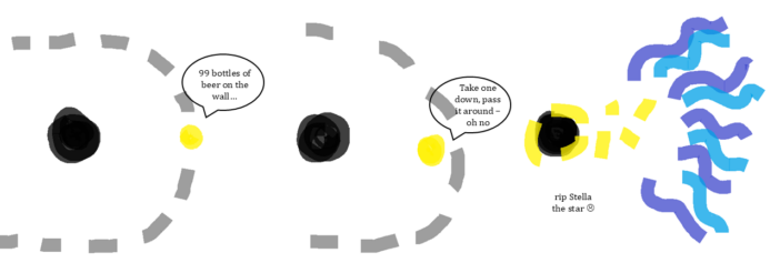
cartoon of a star orbiting a black hole, getting to close, and being ripped apart

Figure 1: Timeline of events leading to a tidal disruption event. [Chloe Klare]

Aside from being cool transients (as far as spectacular stellar deaths go, they are rivaled only by the supernova), TDEs are valuable to study for a variety of reasons. They likely play a role in galaxy evolution, SMBH growth, and even the life cycles of active galactic nuclei (AGN, in which material is constantly swirling onto the SMBH). Not to mention, they are a great tool for eyeballing the mass of the SMBH responsible for the TDE; if the black hole is any bigger than about 1 billion times the mass of the Sun, its event horizon — the point at which not even light can escape its gravity — extends too far, and a star will disappear across the event horizon before it ever gets ripped apart.

How to Spot a TDE

Usually, TDEs are discovered in the X-ray (after all, not many transients are powerful enough to generate an X-ray flare) or in the optical (thanks to high-cadence, wide-field surveys like the Zwicky Transient Facility and the Legacy Survey of Space and Time). However, radio is a particularly useful regime for TDE searches, especially in dusty host galaxies where we cannot see the optical TDE signatures at all; while dust obscures optical light, the radio is unaffected! There is just one catch: how exactly can we identify a TDE based on only its radio emission?

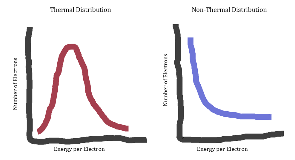
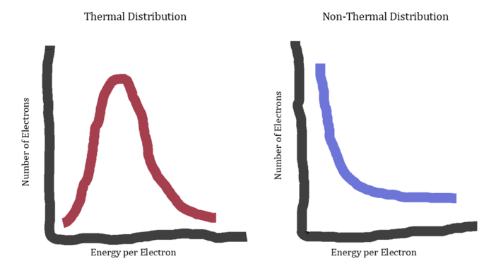
The radio light in a TDE is generated via synchrotron radiation — which is caused by fast moving electrons in strong magnetic fields — and originates in jets or shocks. Unfortunately, this is also the case in AGN, the primary extragalactic source of variable radio emission, and it can be difficult to distinguish between the two. Additionally, the amount of light we see from synchrotron radiation at a given frequency depends on how energy is distributed among the electrons in the source, which is unknown. Perhaps the simplest case — or at least the one you’ll learn about first in your undergraduate statistical mechanics course — is that the energy is distributed among the electrons thermally (left panel in Figure 2). However, most radio transients associated with black holes are assumed to have non-thermal electron energy distributions, usually where there are exponentially many more low-energy electrons than high-energy electrons (right panel in Figure 2).
cartoon showing thermally distributed and non-thermally distributed electrons

Figure 2: Energy can be distributed among the electrons in a source either thermally (left panel), where most electrons have a medium amount of energy, or non-thermally (right panel), where most electrons have a small amount of energy. Often, extragalactic radio transients are assumed to originate from non-thermal electrons, but today’s article argues why we shouldn’t ignore thermal electrons. [Chloe Klare]

As a further challenge, very few TDEs have had extensive follow-up observations in the radio, so we don’t have strong constraints on how most TDEs should behave, especially in the long term. Luckily, some astronomers are working to change this.

This includes today’s authors, who have focused on one particular TDE, ZTF22aaajecp/AT2022cmc (I’m sure everyone mispronounces her name), or 2022cmc for short. 2022cmc is a special TDE: it is one of only five TDEs suspected to have launched a relativistic jet, and it has the highest redshift (z ~ 1.2) of the five. It was observed first in the optical and then in the X-ray and radio. The X-ray emission was highly variable for 400 days post-TDE, and then disappeared, and the first 100 days of radio emission indicated there was a relativistic outflow. At the time, it was concluded that the jet shut off and the X-ray emission ceased. However, the story doesn’t end there; the authors of today’s article continued to observe 2022cmc in the radio for an additional 900 days at frequencies spanning about 1–100 GHz.

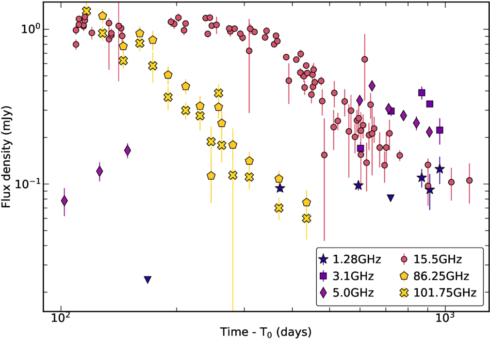
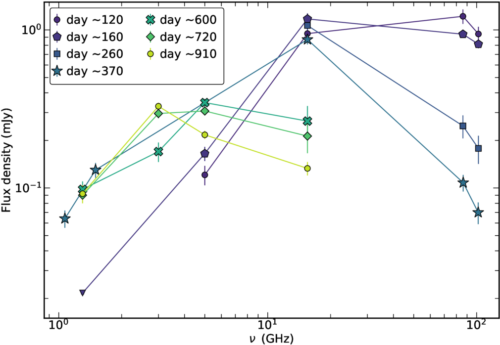
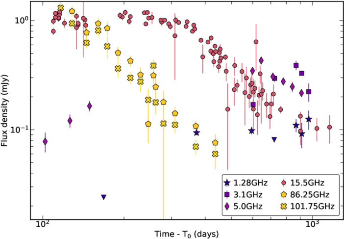
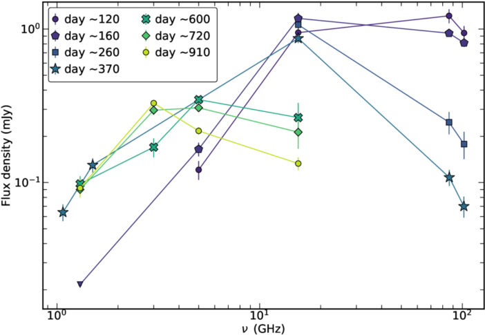
Our authors had two key observing strategies: wide frequency coverage and long duration. Measuring the change in brightness with observing frequency, or the spectral energy distribution (SED), is important for determining which processes are responsible for the radio emission, since thermal electrons and non-thermal electrons will produce different SEDs. On the other hand, measuring the change in brightness over time, or the light curve, is important for determining what is happening at the source, such as whether there is a jet and, if so, how long it lasts. Here, our authors combine light curves at six different frequencies (Figure 3) and SEDs at nine different epochs (Figure 4) to investigate both.
Plot of flux density over time

Figure 3: Light curves spanning six frequencies and 900 days obtained by today’s authors. [Rhodes et al. 2025]
Plot of flux density as a function of frequency

Figure 4: Nine epochs of radio SEDs, which show the peak moving to lower frequencies over time. [Rhodes et al. 2025]

The Findings

Our authors find a couple of interesting results. First, in the time domain, they find the highest-frequency light curves fade with time, while the lower-frequency light curves increase initially, hit peaks at different times (after 300 days at 15.5 GHz, and after 800 days at 1.3 GHz), and then begin to decay. The spectral evolution is even more intriguing; the SED is always peaked, and the peak shifts to lower frequencies over time, which is typical for an expanding emission region. At frequencies below the peak, the SED doesn’t change much. However, the high-frequency side of the SED shows confusing behavior: early on, it has a very steep slope (the amount of light drops off sharply at higher frequencies), but it eventually flattens.

Investigations Begin

Next, our authors consider three possibilities to explain these observations. They first consider synchrotron radiation from only non-thermal electrons in a relativistic jet (Figure 5), which is the canonical model for a gamma-ray burst radio afterglow. Initially, the jet is so fast that all its radio light is relativistically beamed in one direction (like a flashlight), and we can only see the jet if it’s pointed directly at us. Eventually, the jet slows down enough that it is no longer beamed, and light is emitted in all directions (like a light bulb). At this point, we see the light fade over time, which is exactly what happened in the high-frequency light curves. However, there is one glaring problem: this model cannot possibly explain the observed long-lasting steep SED at high frequencies. So, our authors discard this theory.

cartoon showing the jets of a black hole with and without relativistic beaming

Figure 5: The left image shows what a black hole–generated jet looks like in the rest frame of the jet itself. As long as the jet isn’t moving too fast, this is what we see too. However, if the material in the jet is moving near the speed of light, we observe a relativistically beamed jet (right image). [Chloe Klare]

Instead, our authors consider a jetted outflow that has non-thermal and thermal electrons both independently generating synchrotron emission1, giving us the superposition of two radio spectra. This model also doesn’t fit the data well. The peak of the SED moves too slowly, a very dense local environment is required, and, once again, the authors cannot reconcile that steep high-frequency SED.

Lastly, our authors keep the thermal/non-thermal electrons combo and ditch the jet entirely, modeling a spherical outflow. Excitingly, this model best fits the observations, and, most importantly, can explain the mysterious high-frequency behavior. Initially, most of the radio emission originates in the thermal electron population, which produces more light at higher frequencies. As the outflow expands, the non-thermal electrons begin to dominate, and the SED transforms into the classic non-thermal synchrotron shape.

Next Steps

Ideally, our authors want to compare 2022cmc to other TDEs, but few TDEs have such thorough follow-up observations. They speculate that thermal electrons were important in the radio evolution of one of the few such TDEs, Swift J1644, and recommend we revisit its emission models. More broadly, they recommend two future priorities: first, we need extensive radio observations for larger samples of TDEs, especially around 100 GHz, where the thermal electrons contribute most to the SED; secondly, we should stop neglecting thermal electrons not just in TDE models, but in models of any black hole jets, including gamma-ray bursts and X-ray binaries. While this work addresses only one event, one thing is clear. For theorists and observers alike, there is a myriad of exciting work to be done, so it’s no wonder TDEs have garnered so much attention lately.

  1. A convenient property of extragalactic synchrotron sources is that all their electrons radiate independently of one another, even if they are part of the same electron population. This is called incoherent emission. (Galactic sources are another story, but I’ll save that for another time.) ↩︎

Original astrobite edited by Flavia Pascal.

About the author, Chloe Klare:

I’m a PhD student in astronomy and astrophysics at Penn State (with a physics minor, so I get to use my semester spent in QFT for something!). I study active galactic nuclei (in the radio!), and I’m currently looking for baby synchrotron jets in active galactic nuclei.

The post Thermal Electrons Can Explain the Mysterious Radio Behavior of a Tidal Disruption Event appeared first on AAS Nova.

  •  

Long-Term Clustering Pattern of Solar Active Regions and Their Potential Connection with Magneto-Rossby Waves

Junwei Zhao et al 2026 ApJ 1004 175

More than half of solar magnetic flux appears to emerge in three bands, two of which rotate faster than the Carrington rate; this finding suggests a connection between surface flux and interior dynamical processes.

The post Long-Term Clustering Pattern of Solar Active Regions and Their Potential Connection with Magneto-Rossby Waves appeared first on AAS Nova.

  •  

Who Needs Jupiter?

A photograph of Uranus against a black background.

A planned flagship spacecraft to Uranus was aiming to use Jupiter for a gravitational boost to shorten its journey to the outer solar system. Now that the mission’s launch date has been pushed back, it’ll need to find another way to its target.

Redesigning the Route

Uranus and Neptune, the ice giants of our solar system, have been comparatively neglected by humanity’s fleet of interplanetary probes. While all of the other major bodies have been visited by at least an orbiter or even a lander, the most detailed exploration we’ve done of these two planets happened when the Voyager 2 spacecraft went screaming past on its way toward interstellar space.

A two-panel top down view of the solar system with different trajectories overplotted.

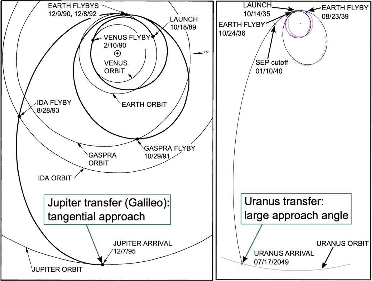
Schematics of different trajectories within the solar system. Left: The path the Galileo spacecraft took to Jupiter. This path arrived nearly parallel to the planet’s motion. Right: One of the proposed paths to Uranus. This path will intersect the planet’s orbit at a much steeper angle to shorten the flight time. Click to enlarge. [Simon et al. 2026]

So it was no surprise when a panel of scientists and engineers charged with setting scientific exploration priorities between 2023 and 2032 recommended finally sending a spacecraft to Uranus, depositing it into orbit around the planet, and keeping it there for a while to collect data. The study itself suggested a basic design for the mission: a pair of spacecraft, one orbiter and one sacrificial atmospheric probe, collectively weighing about 4,000 kg.

Getting these spacecraft to their destination will be a challenge The thriftiest path to get to Uranus, a trajectory called a Hohmann transfer that’s been used for other missions aimed elsewhere in the solar system, would take 16–17 years. Rather than accept the long wait, the original authors suggested that the mission instead fly toward Jupiter, using the giant planet’s massive gravitational tug to slingshot the spacecraft toward Uranus.

However, this plan relied on Jupiter being in just the right place when the spacecraft approached. This in turn relied on the mission launching sometime in 2031 or 2032: any earlier or later, the slingshot would be aimed in the wrong direction. Now that timelines and budgets have slipped for this flagship mission, hitting this launch window seems unlikely. And, without the boost from Jupiter, the mission will have to cross 20 au of open interplanetary space on its own.

Solar Electric Propulsion to the Rescue

A 3-row figure showing the same interplanetary probe flanked by every-growing sets of solar panels.

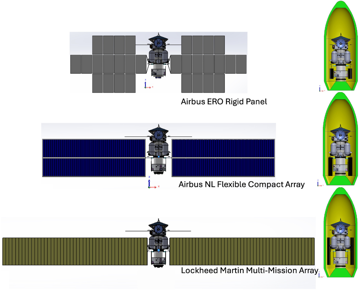
Several proof-of-concept designs for the mission’s SEP components. How these designs would be packaged into a rocket fairing for launch is shown at right. Click to enlarge. [Simon et al. 2026]

Recently, a team led by Amy Simon, NASA Goddard Space Flight Center, took on this challenge and tried to chart a new path through the solar system. The team realized that solar electric propulsion (SEP), a technique that relies on using solar panels to create electricity and accelerate ions to create thrust, might offer a path forward. By using SEP, the mission could leave Earth, unfurl wings of solar panels, then gradually accelerate for as long as there was enough sunlight to power the engine.

The power levels would likely get too low just a few astronomical units into their journey, but that would be enough: after discarding the SEP stage, the mission could coast to Uranus on a journey that would take only 13 years. Even better, this technology has a proven flight history and would require little maturation or development. The BepiColombo mission to Mercury is currently using SEP, and similar techniques are used on satellites in Earth orbit today.

Simon and collaborators also took on a number of other challenges that have cropped up since the mission was proposed, including fewer available plutonium power sources and a re-assessment of Uranus’s rings that revealed hazards in the original flight path. Their work brings the mission closer to the launch pad and illustrates how much iteration goes into the spacecraft that finally takes to the stars.

Citation

“Uranus Orbiter and Probe: Mission Challenges and Concept Updates Since the Origins, Worlds, and Life Decadal Survey,” Amy A. Simon et al 2026 Planet Sci. J. 7 143. doi:10.3847/PSJ/ae680c

The post Who Needs Jupiter? appeared first on AAS Nova.

  •  

Six New Circumbinary Disk Occultation Candidates from the Zwicky Transient Facility

Zhecheng Hu et al 2026 ApJS 284 70

Researchers have identified six new candidate circumbinary disk systems, potentially greatly increasing the number of known systems of this type; these system exhibit deep and prolonged dimming episodes.

The post Six New Circumbinary Disk Occultation Candidates from the Zwicky Transient Facility appeared first on AAS Nova.

  •  

Hydrogen Airglow from an Escaping Ultrahot Jupiter Atmosphere

Yapeng Zhang et al 2026 ApJL 1005 L29

Ultra-hot Jupiter KELT-9b possesses an outflow with a mass-loss rate above 1013 g s-1 — one of the highest mass-loss rates measured for a gaseous exoplanet — and a diagnostic hydrogen Balmer line from its dayside.

The post Hydrogen Airglow from an Escaping Ultrahot Jupiter Atmosphere appeared first on AAS Nova.

  •  

Primordial Planetesimals from the Guts of Population III Stars

Protoplanetary Disk

While previous investigations of planet formation across the universe’s history suggest that planets trickled into the picture, a recent study has found that primordial planetesimals could have formed much earlier from the insides of the first stars in the universe.

First Stars, First Planets?

When the first stars flickered on, the universe was filled with pristine gas, containing only hydrogen, helium, and a little lithium. This gas, though great at making massive stars known as Population III (Pop III) stars, was not yet enriched with the heavy elements necessary for planet formation and, of course, life. Past studies have suggested that planet formation in the universe was gradual, taking several billion years to peak after billions of stars created and spilled the needed metals into the universe. However, local pockets of enriched gas from Pop III stars could have created the right conditions for planet formation earlier in the universe’s history.

Pop III stars burned bright and fast, exploding violently in pair-instability supernovae that completely shredded the progenitor, ejecting over 100 solar masses of metals into their previously pristine surroundings. Cosmological simulations suggest that oxygen from these supernovae could have produced significant water fractions within the dense cores of the supernova remnant. This may have set the stage for planet formation in water-rich disks around subsequent generations of stars as early as 150–200 million years after the Big Bang — does numerical modeling support this planet formation hypothesis?

Protoplanetary disk growth

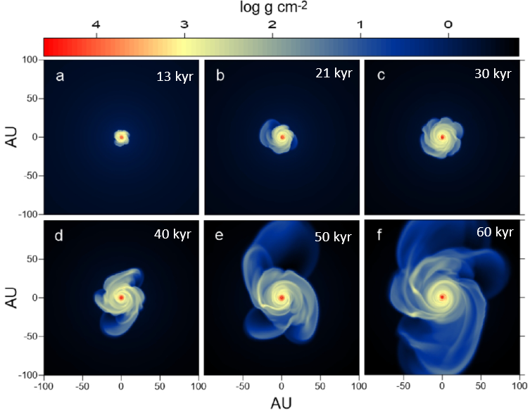
Simulation snapshots showing the formation and evolution of the protoplanetary disk for 13, 21, 30, 40, 50, and 60 thousands of years after protostellar birth. Click to enlarge. [Modified from Vorobyov et al 2026]

Primordial Planetesimals in Simulated Water-Rich Disks

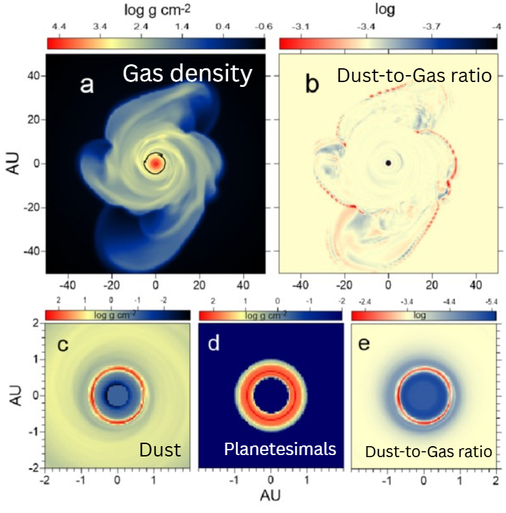
To test if these water-rich dense cores within Pop III supernova remnants could form planetesimals, the building blocks of terrestrial planets, Eduard I. Vorobyov (University of Innsbruck; Southern Federal University) and collaborators performed numerical simulations tracing the collapse of one such gas core into a protoplanetary disk around a protostar. The simulations begin from the gravitational collapse of a 1-solar-mass gas cloud core, with a protostar emerging 24 thousand years after the initial cloud collapse. As the protostar’s gravity pulled in material from its surroundings, a rotating disk formed around the growing star.

Protoplanetary disk evolution and planetesimal growth

Simulation snapshot 40 thousand years after the formation of the protostar showing the gas, dust, and planetesimal surface densities and the dust-to-gas ratio. Click to enlarge. [Modified from Vorobyov et al 2026]

Tracking the gas and dust evolution in the disk, the authors found that several Earth masses of planetesimals formed within 0.5–1.0 au of the 0.4-solar-mass protostar. While the simulations did not trace the disk all the way to planet formation (this requires complex multi-body modeling and lots of computing power), enough planetesimals formed to create a Mars- or Earth-mass planet in the future. Luckily, unlike their live-fast and die-young predecessors, low-mass stars born from Pop III supernova remnants would still be burning hydrogen in their cores today, and ancient metal-poor stars in the Milky Way’s halo may be home to the universe’s first planets that could be detected in future exoplanet surveys. This study showed, for the first time, that water-rich protoplanetary disks with planetesimals could pop up billions of years earlier than previously thought, changing our understanding of planet formation in the universe.

Citation

“Planet Formation at Cosmic Dawn: Planetesimals in H2O-rich Disks around Low-mass Stars,” Eduard I. Vorobyov et al 2026 ApJL 1007 L51. doi:10.3847/2041-8213/ae907c

The post Primordial Planetesimals from the Guts of Population III Stars appeared first on AAS Nova.

  •  

Hitchhiking PAHs Caught Catching a Ride on Galactic Winds

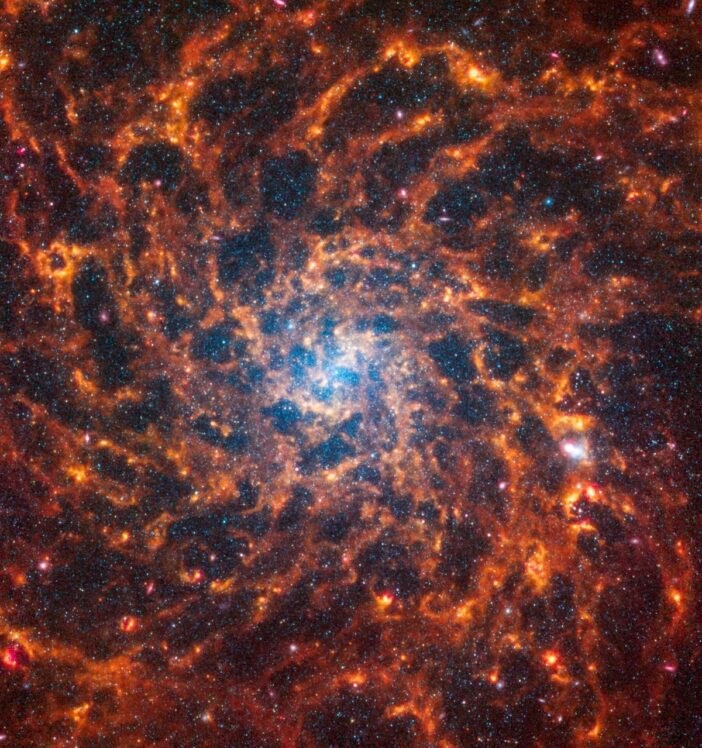
IC 5332

Editor’s Note: Astrobites is a graduate-student-run organization that digests astrophysical literature for undergraduate students. As part of the partnership between the AAS and astrobites, we occasionally repost astrobites content here at AAS Nova. We hope you enjoy this post from astrobites; the original can be viewed at astrobites.org.

Title: JWST Discovery of Warm Dust in the Circumgalactic Medium of the Makani Galaxy
Authors: Sylvain Veilleux et al.
First Author’s Institution: University of Maryland
Status: Published in ApJ

The Windy Galaxy

Billions of light-years away lies Makani, a record-breaking galaxy discovered in 2019 by researchers at the Keck Observatory atop Maunakea, Hawaiʻi. The galaxy shows evidence of a large merger event, where two galaxies collided to form a larger galaxy. This event triggered starburst activity, or several waves of intense star formation, that changed the makeup of not just Makani, but the region around it.

There are several processes that can create galactic winds. An active supermassive black hole at the center of the galaxy can slingshot particles out of the galaxy at close to the speed of light, or supernovae leftover from previous starburst activity can help to expel material from the galaxy. Makani, whose name in Hawaiian just so happens to mean “wind,” has both factors contributing to its galactic winds: massive amounts of star formation and a very active black hole in its center.

This contributes to some of the strongest galactic winds discovered to date, stretching approximately 100 kiloparsecs (330,000 light-years) beyond the galaxy, roughly ten times the extent of a typical galactic wind. These galactic winds remove gas from the galaxy and help to enrich the circumgalactic medium around the galaxy. There is still much to discover about how galactic winds change the makeup of such galaxies, and what exactly they take with them on their way out.

Earth’s Favorite Carcinogen: Polycyclic Aromatic Hydrocarbons

Polycyclic aromatic hydrocarbons (PAHs, pronounced P-A-Hs or “paws”) are small flat dust grains scattered into every corner of the universe, from the atmosphere of Earth in the form of exhaust and wildfire smoke to the circumgalactic medium (the mostly empty space between galaxies). These PAHs contribute to regulating the temperature of the interstellar medium, but astronomers have long wondered how they migrate across galaxies.

Even though they are smaller than a human hair, PAHs are still easily observable even in very distant galaxies.  These dust grains emit infrared light, and if there are enough PAHs in a region, they are bright enough to be observed with modern telescopes, such as JWST. By combining multiple observations across multiple filters, astronomers can calculate ratios that reveal information about the PAHs’ size, temperature, and charge, allowing reserachers to further discern properties about the regions in which these PAHs reside.

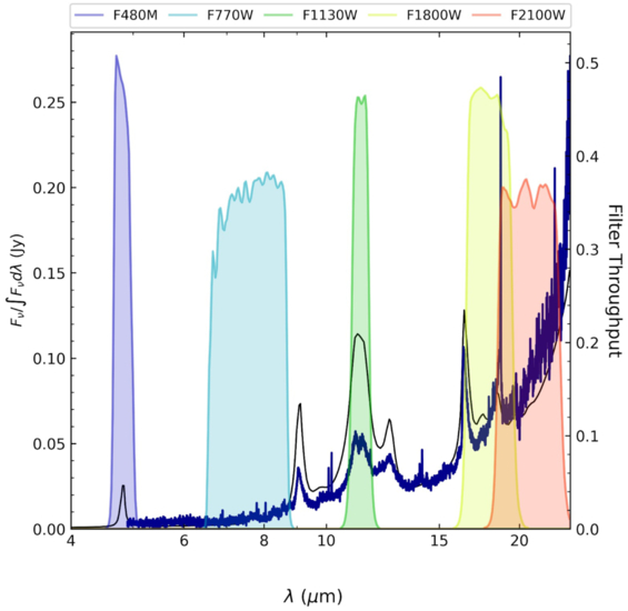
With redshifted galaxies like Makani, the light from PAHs is stretched beyond its usual wavelength, but fortunately for today’s authors, the light was stretched just enough to land known PAH features well within JWST filters, as seen in Figure 1. The authors were then able to use this information to track the distribution of these PAHs across Makani.

JWST spectrum of the galaxy Makani

Figure 1: Makani’s spectrum overlaid on top of the JWST filters. The peaks in the spectrum are PAH features that neatly overlap with JWST’s observing bands. [Veilleux et al. 2025]

PAHs Gone Extragalactic

Using JWST, the authors scrutinized Makani for any signs of PAHs. They found that not only did PAHs exist within the galaxy, these molecules were found up to 30 kpc (~100,000 light-years) outside the galaxy. Makani’s strong galactic winds were ejecting the dust grains from the galaxy over an estimated timescale of a billion years.

Previously, astronomers had not expected to find high quantities of dust grains outside the protection of a galaxy. The journey across a galaxy is long and hot, with temperatures in the millions of degrees. A dust grain would likely not survive the trip, as it would be destroyed by high-energy photons. This suggests that the PAHs were somehow shielded from the hotter parts of the interstellar medium and circumgalactic medium in large enough volumes to make it beyond the edge of Makani.

This answered questions about how galaxies enrich the circumgalactic medium, but it also added several more. Since today’s authors were limited by the sensitivity and range of their instruments, they were unable to confirm if there were PAHs along Makani’s entire wind structure, or just the first 35 kpc (114,000 light-years) of it. They also would like to turn their sights towards the intergalactic medium to see if PAHs could make it even farther beyond the reach of their host galaxy.

Original astrobite edited by Chloe Klare.

About the author, Natalie Price:

As a first-year master’s student at Wesleyan University, I study how stellar winds interact with the local interstellar medium. Outside of the observatory, you can find me dancing, with my nose in a book, or running at non-relativistic speeds.

The post Hitchhiking PAHs Caught Catching a Ride on Galactic Winds appeared first on AAS Nova.

  •  

Smaller Than Earth Habitability Model (STEHM): The Lower Size Limit for Atmosphere Retention in the Habitable Zone

Michelle L. Hill et al 2026 Planet. Sci. J. 7 140

Planets with radii 20% or possibly 30% smaller than Earth’s radius can maintain atmospheres, with initial carbon content, core radius fraction, initial mantle temperature, and other factors playing a role.

The post Smaller Than Earth Habitability Model (STEHM): The Lower Size Limit for Atmosphere Retention in the Habitable Zone appeared first on AAS Nova.

  •  
❌