❌

Normal view

Simulations of Turbulent Mixing Close One Gap but Open Another

6 May 2026 at 17:00

illustration of a white dwarf surrounded by rocky debris

Nature sometimes behaves in ways that are difficult to recreate in simulations. New research tackles the computational challenge of turbulent mixing and rules out a commonly assumed source of data–model disagreement.

Mixing Up Stellar Interiors

What do Earth’s oceans, red giant stars, and white dwarfs have in common? These are all sites of thermohaline mixing, a form of turbulent mixing that takes place when there is a vertical gradient in both temperature and chemical composition. For example, in Earth’s oceans, water near the surface is warmer and saltier than water in the depths below, setting up an unstable situation prone to mixing.

thermohaline mixing simulation results

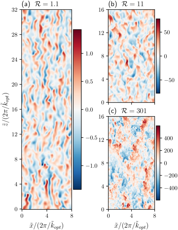
Examples of simulated thermohaline convection. These snapshots show the vertical velocity across a slice through the simulation volume. Click to enlarge. [Fraser 2026]

Thermohaline mixing has been explored in simulations to explain the evolution of red giants’ surface abundances, as well as how quickly rocky debris that accretes onto a white dwarf is absorbed into the star. However, effectively modeling this process in the interiors of stars has proven difficult.

One of the most important parameters for modeling mixing is the Prandtl number, Pr, which is the ratio of viscosity to thermal diffusivity (in other words, a way of describing whether momentum or heat diffuses more quickly within a fluid). For stellar interiors, Pr is around 10−6, but computational limitations have prevented modelers from setting this value lower than around 10−2. When tensions between models and reality arise, this gap between simulated and realistic Pr values is often assumed to be the source of the mismatch.

Bridging the Prandtl Number Gap

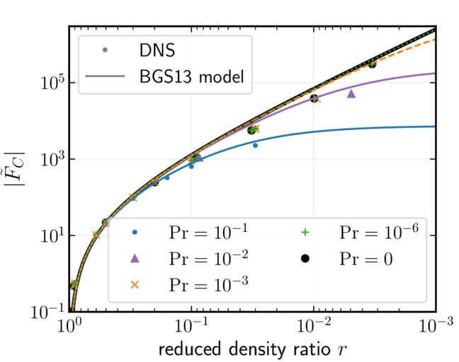
In a recent research article, Adrian Fraser (University of Colorado Boulder) aimed to test this assumption. Fraser carried out 3D simulations of thermohaline mixing, using a semi-implicit modeling technique that lowered the computational cost and allowed the simulations to probe Pr values of 10−1, 10−2, 10−3, 10−6, and 0.

comparison of simulations from this work and the benchmark model of thermohaline convection

Turbulent compositional flux as a function of reduced density ratio for the simulations from this work (DNS) and the benchmark model of thermohaline convection (BGS13). Click to enlarge. [Adapted from Fraser 2026]

By comparing these results against a benchmark model of thermohaline mixing, this exploration showed that adopting a realistic value of Pr doesn’t dramatically change the dynamics of the system — meaning that data–model incompatibilities can’t be swept under a Prandtl number–shaped rug and must instead be resolved by including additional physics.

Recreating Reality

Where does this leave modelers attempting to recreate the reality of stellar interiors? First, a silver lining of this investigation: Fraser found that setting Pr = 0 delivered nearly identical results to Pr = 10−6. This suggests that valid results can be attained in a much less computationally intensive way, since setting Pr = 0 lowers the complexity of the simulation. While simulations with Pr = 0 may not be appropriate for all scenarios, including systems with strong magnetic fields, it may provide a way forward in certain situations.

For modeling of red giants and white dwarfs, Fraser suggested that incorporating magnetic fields, stellar rotation, or additional sources of mixing may resolve the current discrepancies. In fact, some modeling work has shown that magnetic fields could entirely close the gap between observations and models for red giant surface abundances — suggesting that bringing models and observations into agreement may be within reach.

Citation

“Bridging the Prandtl Number Gap: 3D Simulations of Thermohaline Convection in Astrophysical Regimes,” Adrian E. Fraser 2026 ApJL 1001 L22. doi:10.3847/2041-8213/ae5796

The post Simulations of Turbulent Mixing Close One Gap but Open Another appeared first on AAS Nova.

In or Out? Using Balmer Emission to Distinguish Inflows from Outflows

1 May 2026 at 17:00

M33

Galaxies pull in and pump out gas as they form and evolve, but distinguishing between the two directions is tricky. A recent study used emission lines and dust absorption to try to pin it down.

Inflow or Outflow?

Throughout their lives, galaxies churn gas into stars, stars fuse new metals, supernovae blow enriched material back out, and the cycle repeats. To maintain this process and sustain star formation, a galaxy must fuel up by accreting gas from its surroundings. However, catching galactic gas accretion has proven difficult — both emission from gas falling into the galaxy (inflows) and gas blown out by supernovae (outflows) can appear blueshifted or redshifted along an observer’s sight line, depending on if the flowing material is in front of or behind the galaxy.

While direct evidence of inflows has been identified in the Milky Way, only a few direct detections of inflowing gas in other galaxies exist due to the degeneracy of inflow and outflow emission-line features. Relying on additional absorption measurements, some studies have teased out inflows in other galaxies, but these star formation fuel pumps remain overwhelmingly evasive. The angle at which we observe a galaxy also limits our ability to detect both inflows and outflows, with face-on galaxies best oriented to detect these shifted spectral features. How then do we uncover this critical component of a galaxy’s evolution?

Breaking Through with the Balmer Decrement

Balmer decrement diagram

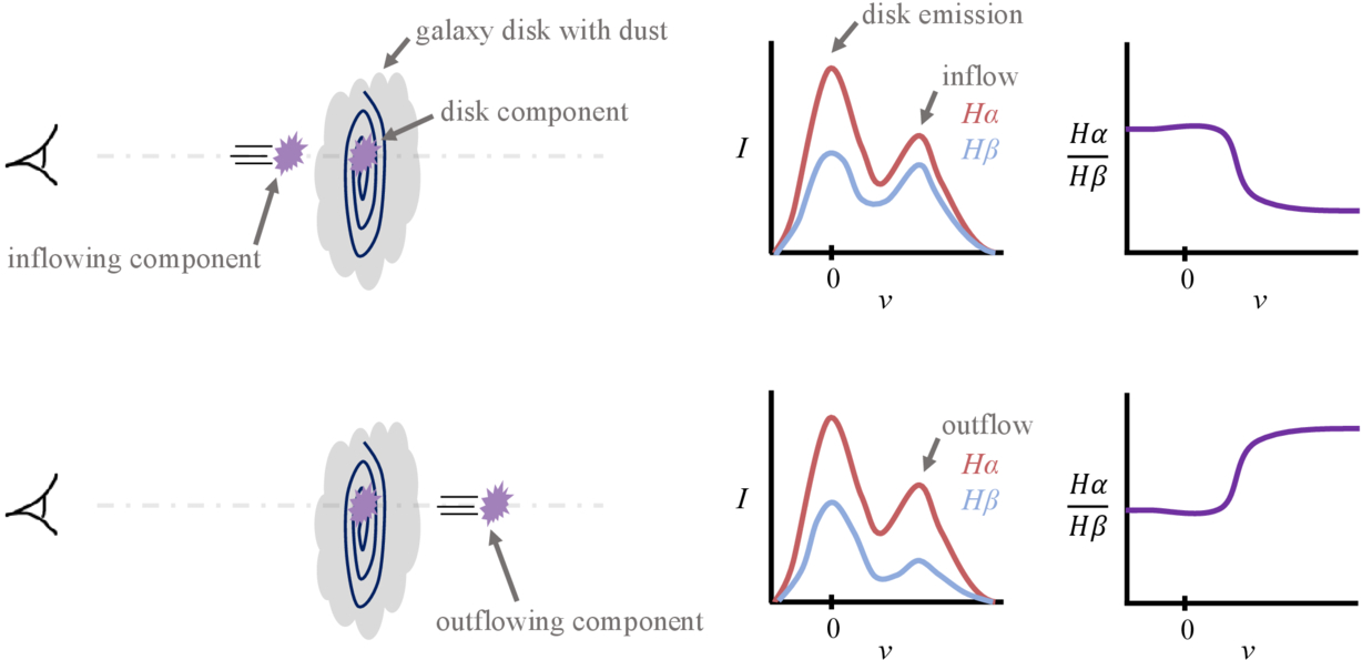
A diagram illustrating the degeneracy in emission spectra of galaxies, with the top panel showing an inflowing component and the bottom panel showing an outflowing component. While the Hα emission is similar, the Hβ emission is more affected by extinction due to dust in the galaxy’s disk, making it possible to identify inflow versus outflow based on the Balmer decrement. Click to enlarge. [Sitaram et al 2026]

To try to break through the confusion between inflows and outflows, Meghna Sitaram (Columbia University) and collaborators explored how the strengths of hydrogen emission lines vary depending on the location of the emitting gas. Referred to as the Balmer decrement, the ratio between the Hα (redder) and Hꞵ (bluer) emission lines is sensitive to dust between the emitting gas and the observer. Because dust preferentially absorbs bluer photons, an inflow or outflow behind a galaxy is expected to have a higher Hα/Hꞵ ratio due to the intervening dust in the galaxy’s disk absorbing some of the Hꞵ emission.

Testing this idea, the authors performed a hydrodynamic simulation of an isolated, face-on Milky Way–like galaxy and tracked inflows and outflows over a billion years. From the simulation, they extracted mock spectral observations to measure the ionized gas motions and Hα and Hꞵ emission lines along different sight lines throughout the galaxy. Separating gas components into three categories — inflow, outflow, and in the disk — the authors found that dust extinction does cause noticeable differences in the Balmer decrement depending on a component’s location with respect to the disk.

histograms

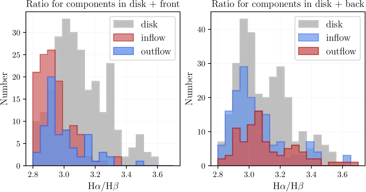
The distribution of Balmer ratios between different components in the interstellar medium and in front of the galaxy (left) and behind the galaxy (right). Material in front of the galaxy shows lower Hα/Hβ ratios. Click to enlarge. [Sitaram et al 2026]

Front Inflow Finds

What does this mean for identifying the inflows that provide galaxies with star-forming fuel? The authors reported that components in front of the galaxy — redshifted inflows and blueshifted outflows — tend to exhibit lower Hα/Hꞵ ratios compared to components behind the disk, aligning with the expectation that dust in the disk absorbs Hꞵ. In particular, these front inflows appear to be the most readily distinguished from gas in and behind the galaxy’s disk.

However, things get more complicated for gas behind the galaxy. Because the dust in the simulation is distributed nonuniformly in small clumps throughout the galaxy, it is difficult to distinguish between disk gas and gas behind the galaxy. While future simulations with improved dust modeling are necessary to resolve this issue, this study offers a useful method to distinguish inflow and outflow in dusty face-on galaxies.

Citation

“Identifying Signatures of Inflow onto Face-On Galaxies Using Balmer Decrement,” Meghna Sitaram et al 2026 ApJ 1001 87. doi:10.3847/1538-4357/ae5222

The post In or Out? Using Balmer Emission to Distinguish Inflows from Outflows appeared first on AAS Nova.

I Survived a Type Ia Supernova, and All I Got Was This Kick Velocity

17 March 2026 at 16:00

G272.2-3.2

Editor’s Note: Astrobites is a graduate-student-run organization that digests astrophysical literature for undergraduate students. As part of the partnership between the AAS and astrobites, we occasionally repost astrobites content here at AAS Nova. We hope you enjoy this post from astrobites; the original can be viewed at astrobites.org.

Title: Supernova Ia Remnants with M-Dwarf Surviving Companions
Authors: Kuo-Chuan Pan (潘國全), Pilar Ruiz-Lapuente, and Jonay I. González Hernández
First Author’s Institution: National Tsing Hua University
Status: Published in ApJ

Type Ia supernovae are important tools astronomers use to measure distances in space. Despite their important role as “standardizable candles,” their origins remain hotly debated. It’s long been theorized that a Type Ia supernova can develop from one of two pathways: the single-degenerate channel or the double-degenerate channel. In the single-degenerate channel, a white dwarf and a non-degenerate star (such as a red giant or main-sequence star like our Sun) orbit each other in a close binary system. The white dwarf accretes material from the outer surface of the non-degenerate star until it reaches a critical mass and explodes. The double-degenerate channel begins instead with two white dwarfs orbiting each other. Most explosion mechanisms from this channel result in the complete obliteration of the secondary, less-massive white dwarf. However, one theoretical explosion mechanism, called the dynamically driven double-degenerate double-detonation (D6) channel, might allow the secondary companion star to survive an explosion from a double-degenerate Type Ia supernova.

Generally, due to the immense energy from a supernova explosion, we expect these surviving companion stars to be “kicked” away from the blasts at high velocities. Fortunately, astronomers have found evidence of these surviving companion stars. As covered in a previous Astrobite, three hypervelocity white dwarfs have been found in Gaia data and traced back to the locations of double-degenerate Type Ia supernovae. Given the prevalence of Type Ia supernovae, however, astronomers are led to question why we haven’t seen many more of these candidates. It’s additionally important to wonder what similar “runaway” companions might look like for the single-degenerate channel.

Recent observations by the Gaia spacecraft near the supernova remnant G272.2-3.2 show an M-dwarf star, MV-G272, with an unusually high velocity around 240 km/s and a trajectory tracing back to the center of the supernova remnant. Is it possible for this M dwarf to be the runaway companion to the remnant’s original supernova? The authors of today’s article look at simulations of potential companion stars from single-degenerate Type Ia supernovae and compare their results to this observed potential companion candidate.

Because this work focuses on the potential for M-dwarf companions, the authors explored a range of simulated companion-star masses and radii characteristic of M dwarfs: 0.5, 0.6, and 0.7 solar mass and 0.396, 0.454, and 0.483 solar radius, respectively. To make these models, they used the stellar evolution code Modules for Experiments in Stellar Astrophysics (MESA) to construct and evolve a number of simulated stars with these specifications.

After setting up the models in MESA, they used the magnetohydrodynamics code FLASH to perform 2D and 3D simulations of the supernova explosion and the subsequent impact of the exploding star’s ejecta (or hot material) on its M-dwarf companion. After the explosion and impact were modeled, the companion star’s evolution was further followed in MESA.

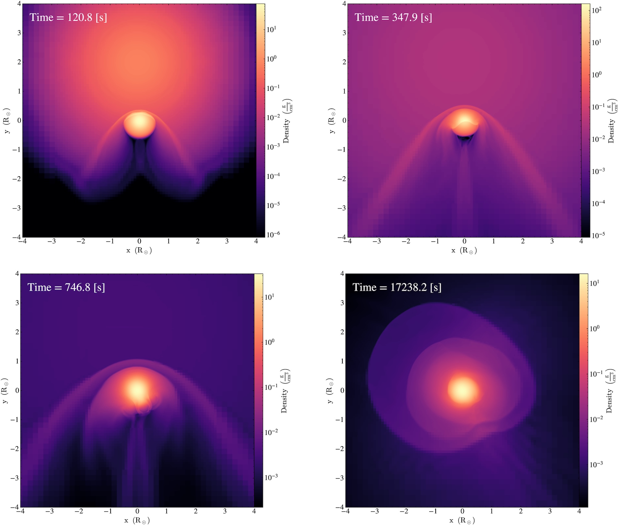
Figure 1 shows the density of the supernova’s ejecta, or exploding material, as it impacts the companion star. (You can think of this figure as if you were looking at the companion star out in space.) After roughly 100 seconds, you can see a bow shock develop around the top of the companion (or the “front” of the star) as it wraps around the companion. This impact causes significant compression of the companion star and rips away upwards of 50% the companion’s mass. The impact of this shock is what gives the companion star its “kick,” sending it hurtling through space.

simulations of supernova ejecta colliding with a star

Figure 1: Visual of the density of the companion star (center of each plot) and the supernova ejecta over time. In the top row of plots and the bottom-left plot, you can see the higher-density bow shock bent around the top (or front) of the companion star. In the bottom-right plot, you can see some of the supernova ejecta and unbound mass from the companion star settling around the companion star. [Pan et al. 2025]

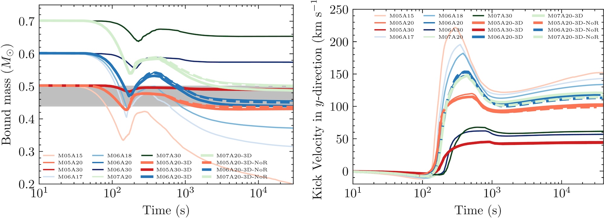
Because the authors explored a range of initial companion masses and distances between the primary and companion star, their results show some range. Figure 2 shows two important results: the evolution of the companion’s mass before and after the explosion (left plot), and the evolution of the companion’s kick velocity (right plot). The dip in mass around 100 seconds (102 s) indicates the impact of the bow shock. Even though the simulations model companions with a relatively narrow mass range (0.3–0.7 solar mass), there is considerable variation in the final masses after explosion. For example, the initial 0.5-solar-mass model ends up with anywhere between 0.07 solar mass (just 14% of its initial mass) and almost its full initial mass of 0.5 solar mass, depending on the distance between the companion and its exploding star.
plots of bound mass and kick velocity as a function of time

Figure 2: The different models shown in both plots indicate different initial masses and separation distances between the companion and the exploding star. Left: how the companion’s gravitationally bound mass evolves over time. The plot can be read left to right. The dip around 102 seconds indicates the impact of the supernova shock, which unbinds layers of the companion’s mass. Some of that mass becomes bound again to the companion after the shock passes. Right: how the companion star’s kick velocity changes based on initial mass and separation distance between companion and exploding star. The peak in values between 102 and 103 seconds indicates the impact, or “kick,” from the supernova. [Pan et al. 2025]

The results from this work generally show, predictably, that a companion closer to its primary star gets a bigger kick in velocity. These “kicks” range from about 50 km/s to 150 km/s. When added to the system’s initial velocity in space, it brings the total velocity of these companions into the 150–200 km/s range. This result is generally well aligned with the observed velocity of MV-G272, which was roughly 240 km/s.

Notably, runaway companion stars of these Type Ia supernovae seem to retain information from the initial explosion. Given the final velocities of these companions, astronomers might be able to figure out the companion’s initial mass and trace back its trajectory to the system it originated from. Overall, the fact that MV-G272 has a trajectory that tracks back to the center of a supernova remnant makes it a good companion candidate. These results support the feasibility of M-dwarf runaway companions from single-degenerate Type Ia supernova systems. Now that we know what these companions might look like — and how fast they can be going — astronomers can hopefully better search for these high-velocity stars in the future.

Original astrobite edited by Catherine Slaughter.

About the author, Mckenzie Ferrari:

I’m currently a PhD student in the geophysical sciences program at the University of Chicago. While I now study the atmosphere and oceans of Earth, most of my previous research focused on simulations of Type Ia supernovae and galaxy formation and evolution. In my free time, I foster cats for a local organization, enjoy cooking, and can often be found running along Lake Michigan.

The post I Survived a Type Ia Supernova, and All I Got Was This Kick Velocity appeared first on AAS Nova.

Ia’m Just Getting Started: A Type Ia Supernova’s First Day

24 February 2026 at 17:00

G299.2-2.9

Editor’s Note: Astrobites is a graduate-student-run organization that digests astrophysical literature for undergraduate students. As part of the partnership between the AAS and astrobites, we occasionally repost astrobites content here at AAS Nova. We hope you enjoy this post from astrobites; the original can be viewed at astrobites.org.

Title: The First Day of a Type Ia Supernova from a Double-Degenerate Binary
Authors: Gabriel Kumar, Logan J. Prust, and Lars Bildsten
First Author’s Institution: University of California, Santa Barbara
Status: Published in ApJ

Much like distance markers along the highway, Type Ia supernovae have long been used as distance indicators in space. These supernovae were originally theorized to form in binary systems. In this system, a white dwarf (a dense, collapsed remnant of a star) steals surface material from a non-degenerate star like our Sun and then explodes. Because of the initial conditions and properties of those two stars, the explosion would shine with the same intrinsic brightness regardless of the binary system’s location in space.

Research and observations, however, show that this is not entirely true; not all Type Ia supernovae are equally luminous. There are various theories regarding the different formation scenarios and explosion mechanisms that might create a Type Ia supernova. Developing ways to sleuth out the origins of these systems can be useful because it may tell us more about their luminosity.

One emerging theory of formation is the “double-detonation scenario.” In this case, two white dwarfs exist in a binary system. The more massive primary (the “accretor”) steals material from the less massive white dwarf secondary (the “donor”). After the primary steals the donor’s outer thin shell of helium, the helium surrounding the accretor detonates. This explosion induces a shock wave that travels into the dense core of the accretor and causes another detonation. The two detonations — one on the surface and one in the core — produce enough energy to explode the star into a supernova, a powerful stellar explosion. When the material from the exploding star reaches its companion star, it forms a mysterious, conical wake within the gaseous material, or “ejecta,” expelled from the accretor. This wake might be an important clue for distinguishing a supernova’s origins.

Since these explosions are incredibly powerful and would be difficult (and dangerous!) to perform in a lab, astronomers turn to computer simulations to model these events. Hydrodynamical simulations, in particular, are helpful for researchers because they model how fluids “flow” by solving complex equations that are too tricky to do by hand. (Remember that stars are just balls of gas, and hence fluid!) The authors of today’s article ran hydrodynamical simulations of the explosion and subsequent evolution of the ejecta from a double-detonation scenario.

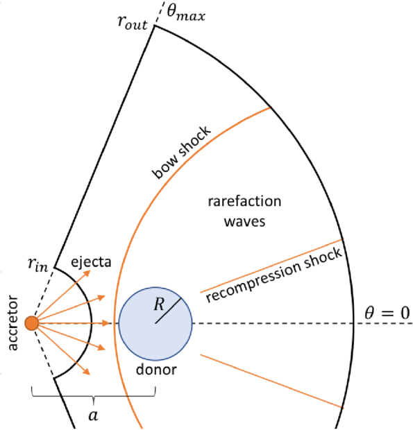
In the diagram of the team’s setup (see Fig. 1), you can see a “bow shock.” This shock is from the wave produced in the accretor’s detonation and is bowed since it bends around the donor star. This shock moves quickly through the cone of ejecta, modifies its structure, and leaves clues within the ejecta as it settles.

schematic of the simulation setup

Figure 1: A visual schematic of the simulation setup. The accretor is the exploding star, which produces a “bow shock” from the detonation. The bow shock and recompression shock modify the structure of the ejecta, which fills the space between rout and rin. The ejecta is full of gaseous stellar material. [Kumar et al. 2025]

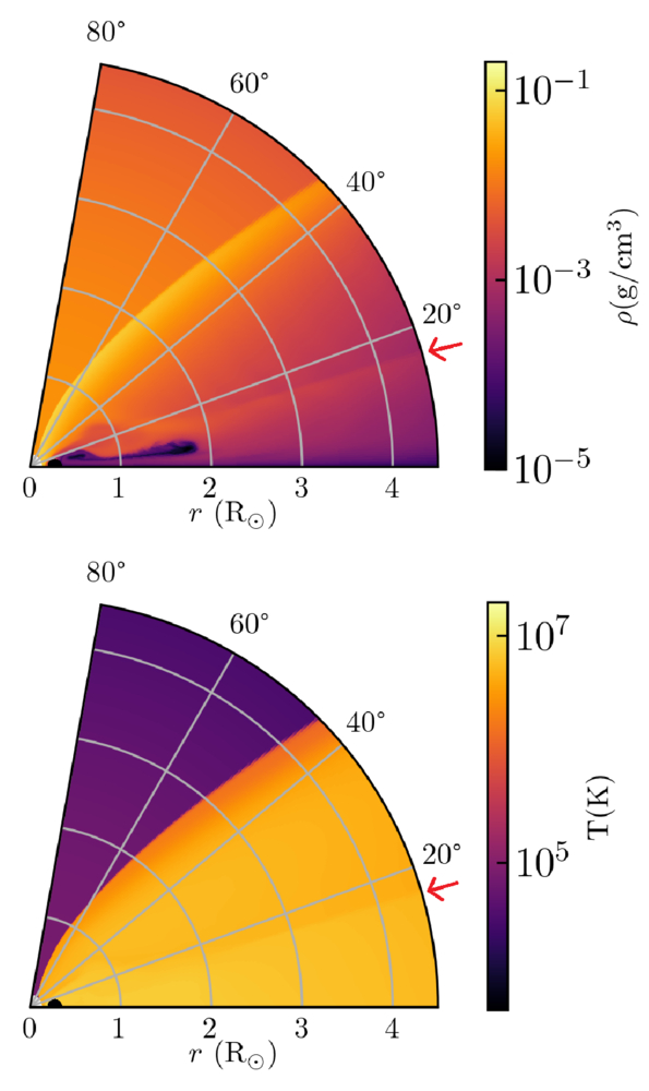
After simulating 1,000 seconds after the explosion, the authors recreated a high-density, low-temperature “wake” from the shock. You can see imprints of this wake in Fig. 2, as denoted by the red arrow.
visual slice of the simulated ejecta

Figure 2: A visual “slice” of the ejecta surrounding the donor star just 200 seconds after detonation. The bottom-left corner (r = 0) has a faint white spot, indicating the donor. The density (top) and temperature (bottom) of the ejecta are shown. The faint line marked by the red arrow indicates the secondary shock from the explosion, highlighting changes in both density and pressure. [Kumar et al. 2025]

Once they were able to produce this wake, the authors evolved the ejecta over time to see what the radiation from this material might reveal. They discovered that the “shocked,” or compressed and heated, ejecta flew out much further than the unshocked ejecta (see Fig. 3).
simulation snapshot at 2 hours of simulation time

Figure 3: A slice of the simulation taken later, at 2 hours of simulation time. The ejecta in the shocked region has flown out farther than the ejecta in the unshocked region. Note that the horizontal scale has changed from Figure 2. [Kumar et al. 2025]

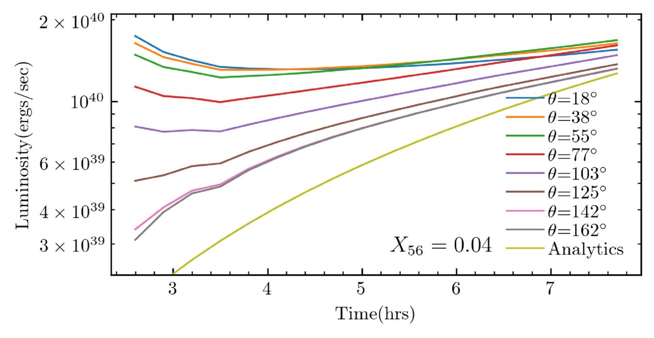
This ejecta can be seen from different viewing angles, influencing an observer’s measurement of the explosion’s luminosity. The strongest features of the wake are visible up to about 55 degrees, while some effects can still be seen up to about 140 degrees — almost half of the sky (see Fig. 4). Overall, an observer’s position relative to the explosion axis might change their reported luminosity of the explosion. The authors estimate that this wake might cause Type Ia supernovae from a “double-detonation” scenario to appear up to 15% fainter, depending on the observer’s viewing angle. Therefore, if scientists use Type Ia supernovae as cosmic distance indicators, their calibrations might be slightly off. This isn’t the best news for those using measurements of Type Ia supernovae to measure the expansion rate of the universe.
plot of luminosity versus time after detonation of a supernova

Figure 4: A comparison of luminosity vs. time over the course of 6 hours shortly after detonation. The different lines indicate different viewing angles from the axis of explosion. The line “Analytics” describes a light-curve prediction by Piro (2012) for a supernova that was not shock-heated. The luminosities for this model span almost one order of magnitude. [Kumar et al. 2025]

We’ve talked a lot about the accretor and ejecta in this scenario, but what might happen to the donor star? One idea is that the donor star is “kicked” away by the high velocity of the blast. In this simulation, the authors were able to calculate a “kick” velocity, or speed imparted by the blast to the donor star, that was much higher than estimates from other detonation models. One observed Type Ia supernova, SN 2021aefx, is believed to have the fastest observed ejecta to date. The mechanism that today’s authors modeled might explain how the ejecta of this event got its super-fast “kick.”

While there is always more work to be done, this work presents a first step at identifying double-detonation Type Ia supernovae from early observations. With an influx of observations from new observatories, like the Vera C. Rubin Observatory, we should expect to see many more early supernova detections.

Original astrobite edited by Ansh Gupta.

About the author, Mckenzie Ferrari:

I’m currently a PhD student in the geophysical sciences program at the University of Chicago. While I now study the atmosphere and oceans of Earth, most of my previous research focused on simulations of Type Ia supernovae and galaxy formation and evolution. In my free time, I foster cats for a local organization, enjoy cooking, and can often be found running along Lake Michigan.

The post Ia’m Just Getting Started: A Type Ia Supernova’s First Day appeared first on AAS Nova.

Scars from a Black Hole

10 September 2025 at 17:00

A spiral of bright material circling a black core.

Simulations suggest that there should be a million stars in our galaxy that once wandered so close to a supermassive black hole that they were nearly destroyed. What are the long-term effects of this encounter, and could astronomers observe the scars of these near-death experiences?

Moths to a Flame

center of the Milky Way

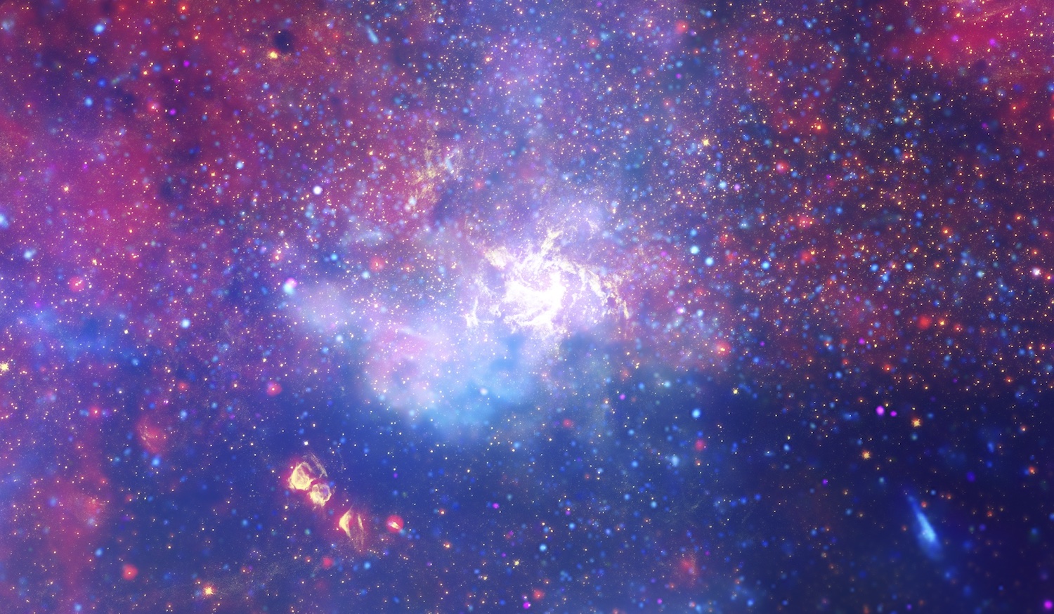
This infrared and X-ray image of the Milky Way’s center shows a swirl of hot gas surrounding Sagittarius A*, our galaxy’s central supermassive black hole. [NASA, ESA, SSC, CXC, STScI]

The center of our galaxy is a dangerous place to be a star. Like mosquitoes drawn to a light, millions of stars swarm around the supermassive black hole named Sagittarius A*, packing themselves in tight and kicking one another onto wild, eccentric, and ever-changing orbits. Every 100,000 years or so, one of these stars gets an unlucky push and finally gives in to the black hole’s irresistible pull. A nudge from a neighbor will send it hurtling beyond the point of safety, and in one intense flyby, it’ll be ripped apart by Sagittarius A*’s immense gravitational field.

Simulations suggest that most of the time, these hapless stars are not completely destroyed by their close encounters with the black hole. In principle, then, there should be about a million “survivor” stars wandering near the center of our galaxy. But, what would these survivors look like? And with careful measurements, could we tell them apart from their regular, unscathed counterparts?

Simulating a Star’s Worst Day

Recently, a team of astronomers led by Rewa Clark Bush (University of California Santa Cruz, Cabrillo College, Wesleyan University) tackled this question. First, the team needed to simulate a terrible day for a hypothetical star: the day it passes closest to the black hole. To compute what happens to the star in those intense couple of hours, they used an open-source hydrodynamic code called FLASH to track the state of the star in granular detail.

An 8-panel figure showing complex, asymmetric patterns of gas around a dense core.

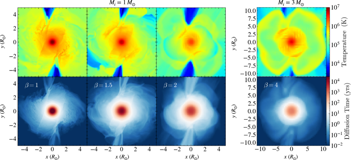
Temperatures (top row) and diffusion timescales (bottom row) of four stars soon after their closest approach to the black hole. Click to enlarge. [Bush et al. 2025]

Then, once the star (or what was left of it) managed to flee back to safety, the team froze the simulations and took stock. They found that depending on the initial size of the star and the distance of its closest approach, the black hole stripped away anywhere from a few percent to almost two thirds of the star’s mass. The researchers then fed the stars into another code called MESA to simulate how the disturbed stars would settle into a new equilibrium and evolve over billions of years.

Back on Track

Plot comparing disturbed and undisturbed stars

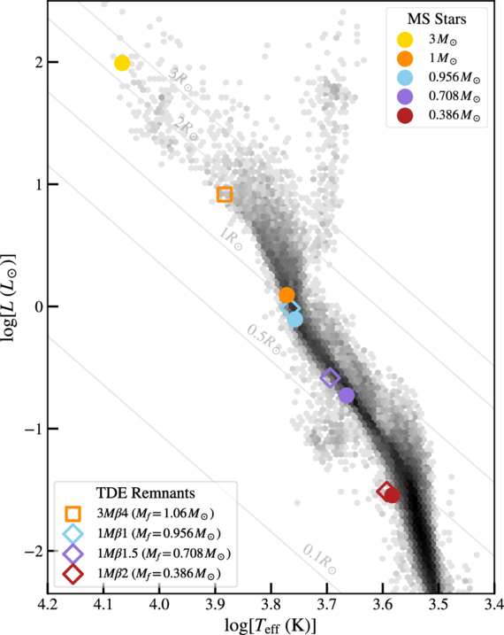
Comparison of the original undisturbed stars (filled circles), the stars after a black hole encounter (open symbols), and other stars with different initial masses (black points). Click to enlarge. [Bush et al. 2025].

The team found that although these unlucky stars likely glow tens to hundreds of times brighter than usual after their flyby, this period of enhanced brightness lasts less than 100,000 years. For our galaxy, this translates to 1–10 stars currently in the galactic center that have been brightened by an encounter with a supermassive black hole.

Eventually, though, these stars pretty much return to a new normal. Though these stars would have had slightly different colors and luminosities had they not encountered the black hole, they end up looking similar to undisturbed stars with the same final mass.

Although detailed spectroscopic measurements of these remnants might reveal a strange composition thanks to all the stirring that happened during the flyby, it’d be hard to tell anything happened to these stars otherwise. Ultimately, life goes on, even for stars that were nearly destroyed by the most massive creature in the galaxy.

Citation

“Black Hole Survival Guide: Searching for Stars in the Galactic Center that Endure Partial Tidal Disruption,” Rewa Clark Bush et al 2025 ApJL 990 L7. doi:10.3847/2041-8213/adefde

The post Scars from a Black Hole appeared first on AAS Nova.

Escaping the Dust Trap: Simulations of Dust Dynamics in Protoplanetary Disks

25 July 2025 at 17:00

Through detailed simulations of gas and dust, a recent study revealed that the behavior of dust within protoplanetary disks is a bit more complex than previously assumed.

Dust Traps in Protoplanetary Disks

As a planet forms within a protoplanetary disk — dust and gas orbiting a new star — tidal interactions between the budding body and the dusty material surrounding it can create pressure bumps where dust builds up. These dust traps appear as rings in observations of protoplanetary disks.

Dust traps are thought to play a critical role in the disk’s evolution and the early stages of planet formation. Dust traps may prevent solid material from migrating inward, starving the inner disk and impeding planet growth interior to the trap. These reservoirs may also serve as a chemical barrier, keeping volatile materials like water from moving to the inner regions of a disk.

While a perfect dust trap completely isolates material from the rest of the disk, recent observations and 2D simulations have shown that dust traps may be a bit more permeable — leaking smaller sized grains, mixing material, and changing the disk’s appearance. However, these results only account for two dimensions of the complex three-dimensional environment in which dust traps reside. Thus, 3D hydrodynamical simulations are necessary to provide more realistic details of dust dynamics within planet-hosting protoplanetary disks. 

Dusty Simulations

Dust-gas density ratios for 3d models at 1500 orbits

Z-axis averaged dust–gas density ratios (top) and dust–gas surface density ratios for the 3D simulations after 1,500 orbits. For the simulations with higher diffusion and lower planet mass, there is clear leaking of dust beyond the dust trap ring (edges marked with dotted red lines). Click to enlarge. [Huang et al 2025]

In a recent study, Pinghui Huang (Chinese Academy of Sciences; University of Victoria) and collaborators performed multiple 2D and 3D numerical simulations of gas and dust within a protoplanetary disk with a forming planet. The simulations varied the mass of the planet and the level of turbulent diffusion — how well material and energy flow and mix within the gas. These variations allowed the authors to explore how dust traps behave within different types of systems. 

The simulations showed that the embedded planet will perturb the gas and dust, producing density shocks that create gaps and, subsequently, pressure bumps where dust traps coalesce. From their analysis, the authors found that dust traps become leakier at higher levels of diffusion and when the embedded planet is lower in mass. Essentially, if the gas flows and mixes more efficiently, the perturbations of the planet are erased more quickly, and if the planet is sufficiently small, its ability to disrupt the disk is much weaker. Dust remains coupled to the gas, flowing through these weak traps without becoming stuck. Additionally, the 3D simulations show higher amounts of leakage compared to the 2D simulations, which the authors attributed to the asymmetric and complex vertical geometry of the disk.

Trapping over time.

Flux-trapping ratio (left) and mass-trapping ratio (right) as a function of time for the 2D (top) and 3D (bottom) simulations. The higher-mass planet in Model A causes more flux and mass-trapping than the lower-mass planets and more turbulent systems. Additionally, the 3D simulations show significantly lower flux and mass-trapping than the 2D simulations. Click to enlarge. [Huang et al 2025]

Implications and Comparison to Observations

What then are the consequences of leaky dust traps? In planet formation theory, dust traps determine the mass at which a planet creates a sufficient pressure bump that isolates small pebbles and dust exterior to its orbit. For perfect dust traps, this isolation of material from the planet and inner disk creates a clear chemical distinction between the inner and outer disk. However, as shown by the 3D simulations, dust traps are imperfect, allowing small particles to filter through; the authors suggest this may mean that the growing planet slows but does not stop the migration of solid materials in a disk.

Recent observations of protoplanetary disks reveal the presence of larger volatiles within the inner disk. Specifically, the disk PDS 70 shows water emission in its inner disk despite having two confirmed giant planets orbiting in the outer disk. Without leaky dust traps, volatiles like water would be trapped in the pressure bumps created by these planets. However, as the authors have shown, the complex reality of dust dynamics within protoplanetary disks allows heavier elements to leak through, enriching the inner disk. Further observations and detailed 3D simulations will allow astronomers to understand the extent of leaky dust traps and reveal the realistic conditions driving early planet formation.

Citation

“Leaky Dust Traps in Planet-Embedded Protoplanetary Disks,” Pinghui Huang et al 2025 ApJ 988 94. doi:10.3847/1538-4357/addd1f

The post Escaping the Dust Trap: Simulations of Dust Dynamics in Protoplanetary Disks appeared first on AAS Nova.

❌